Introduction to Hypothesis Testing
Lecture 8
NC State University
ST 511 - Fall 2024
2024-09-11
Checklist
– Keep up with Slack
– AE Solutions Posted
– Quiz 2 Solutions Posted
– HW-2 Posted Today ~ 5:00 (due Monday 23rd)
– HW-1 Solutions (today; grades soon)
Announcements
Quiz 3 - Question 3
The Central Limit Theorem states that we always need to have at least a sample size of at least n = 30 for the sampling distribution of a sample statistic to be approximately normal.
\(\geq 30\) vs \(> 30\)
The literature is sloppy (and apparently so am I)
Both is fine. I’m going to be more consistent with \(> 30\)
Warm Up Question
Notation check
\(\hat{p}\)
\(\mu\)
\(\bar{x}\)
\(\pi\)
Warm Up Question
Notation check
\(\hat{p}\) - sample proportion
\(\mu\) - population mean
\(\bar{x}\) - sample mean
\(\pi\) - population proportion
Warm Up Question
Suppose you are a researcher interested in studying food habits for NC State students. You take a random sample of 100 students, and are interested in if they had Howling Cow ice creme with their dinner or now. We observed 37 students have ice creme, and 63 students not have ice creme.
– What is our random variable (X)?
– What type of variable are we working with?
Warm Up Question
Suppose you are a researcher interested in studying food habits for NC State students. You take a random sample of 100 students, and are interested in if they have Howling Cow ice creme with their dinner or now. We observed 37 students have ice creme, and 63 students not have ice creme.
We know that the Central Limit Theorem works with means (under certain conditions). Can X be represented as a mean?
Warm Up Question
\[ X = \begin{cases} 1 & \text{if yes}\\ 0 & \text{if no} \end{cases} \]
1, 0, 1, 1, 0, 1, 0, 1, …..
The mean of a binary outcome is just the sample proportion
Procedures
Do Students Eat Howling Cow?

– Set up your null and alternative hypothesis
– Collect data
– Quantify evidence
– Articulate your results
Do Students Eat Howling Cow?

Suppose the Howling Cow company claims that 50% of NC State students eat Howling Cow at dinner. We think that less than 50% of students eat Howling Cow at dinner.
\(H_o\): - The assumption that is made
\(H_a\) - The research question
Do Students Eat Howling Cow?
\(H_o\): \(\pi\) = 0.5
\(H_a\) \(\pi\) < 0.5
\(>\)
\(\neq\)
Collect Data
You take a random sample of 100 students, and are interested in if they have Howling Cow ice creme with their dinner or now. We observed 37 students have ice creme, and 63 students not have ice creme.
What is the proper notation for our sample statistic?
Collect Data
You take a random sample of 100 students, and are interested in if they had Howling Cow ice creme with their dinner or now. We observed 37 students have ice creme, and 63 students not have ice creme.
What is the proper notation for our sample statistic?
\(\hat{p}\) = \(\frac{37}{100}\)
Null Distribution
A null distribution is a sampling distribution under the assumption of the null hypothesis. It describes how that statistic would vary from sample to sample, if the null hypothesis were true.
We can use theory or simulation techniques to model this distribution if our assumptions hold!
Theory Based Methods
Assumptions for single proportion
– Independence (this never goes away)
– Sample size (a little different than with means)
Sample Size Assumption
– Need to think about the number of successes + failures
– Need to think about creating a sampling distribution under the assumption of the null hypothesis
– \(\pi = 0.5\)
So we ask ourselves, if the null is true, how many successes and failures would we expect to see out of our sample size of 100?
Sample Size Assumption
n = 100
Success = 0.5
100*.5 = 50
Failure = 0.5
100*.5 = 50
Estimating the sampling distribution
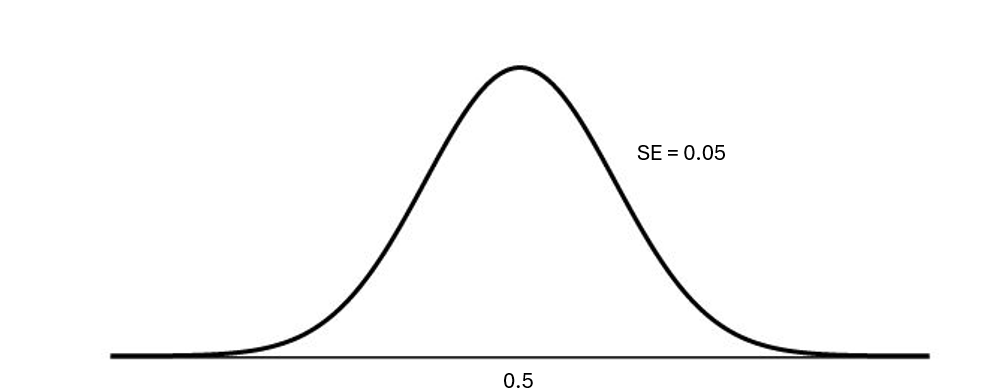
The null value will be the center
We can estimate the standard error of the null sampling distribution as so:
\[ \sqrt{\frac{\pi_o * (1-\pi_o)}{n}} \]
What this looks like
Standardize
Often, with theory-based methods, we use a standardized statistic. A standardized statistic is computed by subtracting the mean of the null distribution from the original statistic and dividing by the standard error
\[ \text{statistic} = \frac{statistc - null}{SE(null)} \]
Why?
– The standardized statistic has a nice definition
– Helps compare across multiple studies with different units
Standardized test statistc
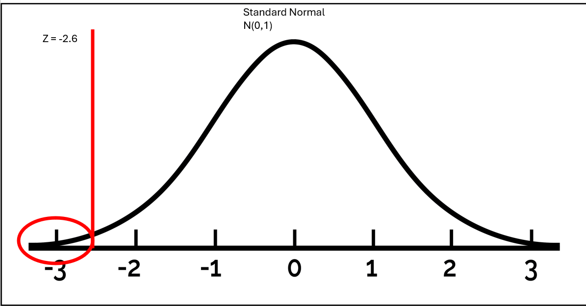
\[ Z = \frac{.37 - .5}{.05} = -2.6 \]
Interpretation - Interpreting this value, we can say that our sample proportion of 0.37 is 2.6 standard errors below the null value of 0.50.
Why Z?
The reason you can use a z-test with proportions is because the standard deviation of a proportion is a function of the proportion itself. With proportions, we assume the standard deviation is known exactly.
Step Back
Under an assumption of some null hypothesis, would you expect to observe this statistic?
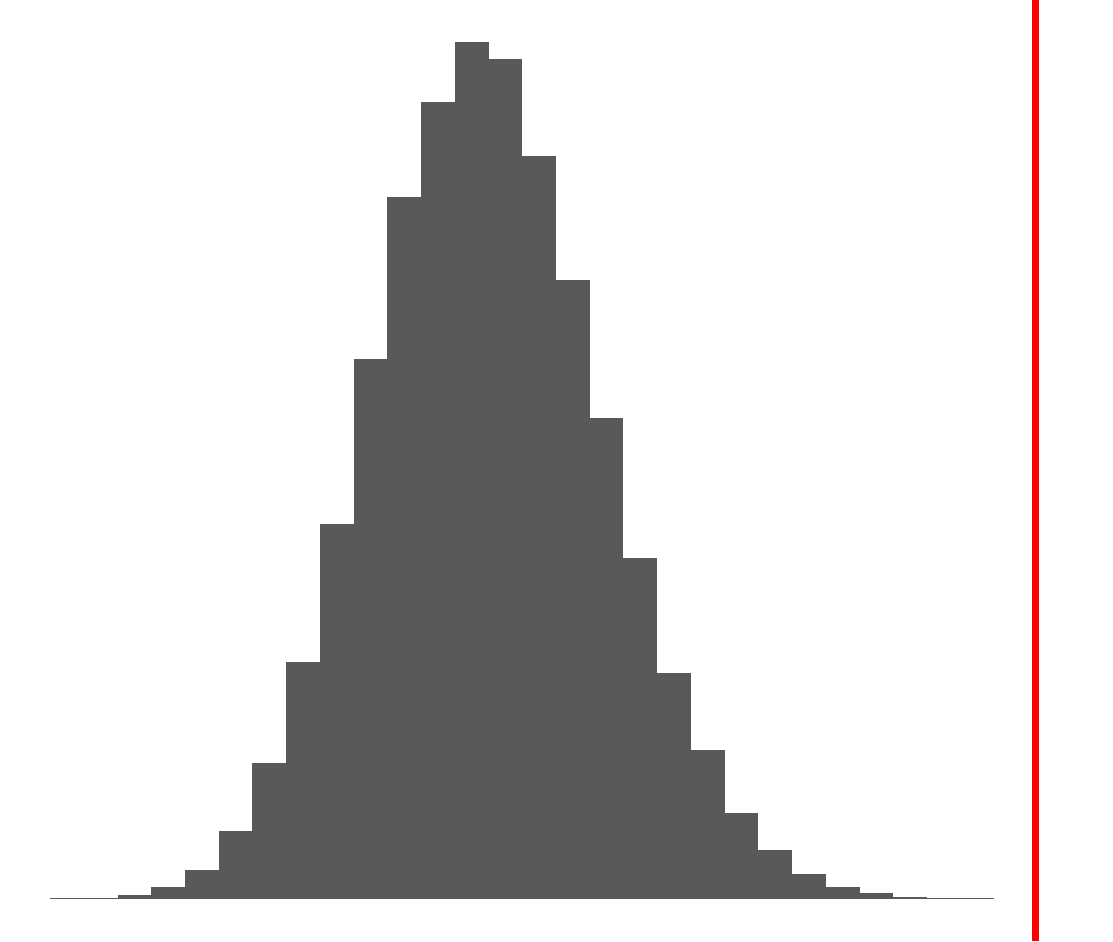
Step Back
Under an assumption of some null hypothesis, would you expect to observe this statistic?
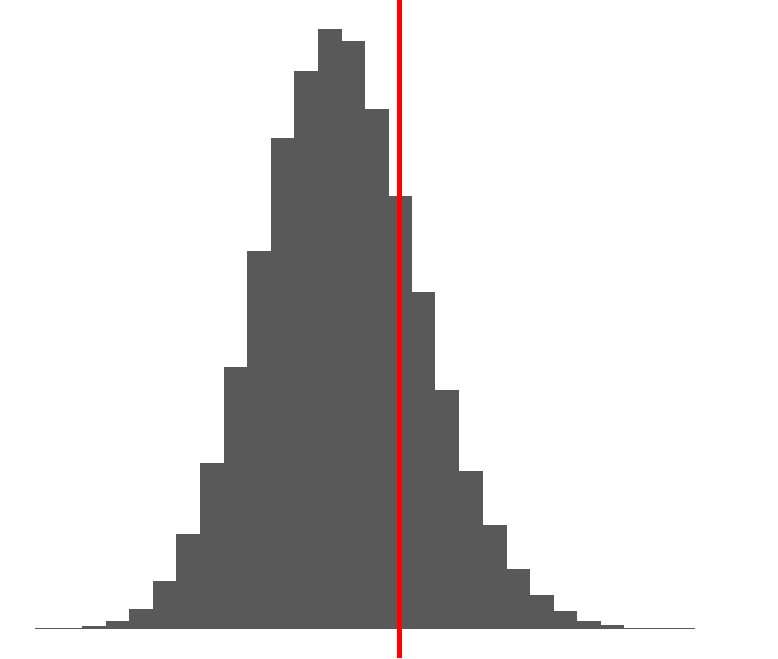
Under an assumption of some null hypothesis, would you expect to observe this statistic?

- Probably not! Let’s quantify that thinking
P-value
A p-value is the probability of observing our sample statistic, or something more extreme given our null hypothesis is true
Let’s fill in the bold with our context!
P-value
A p-value is the probability of observing .37, or something smaller given the true proportion of all NC State students that eat Howling Cow ice creme at dinner is 50%
P-value
pnorm() is used to calculate probabilities from a Normal distribution
arguments:
– quantile (z-statistic of -2.6)
– mean
– sd
– lower.tail = [TRUE/FALSE]
Alpha
\(\alpha\) (also called significance level), acts as a “cut-off” for how much evidence we need to reject the null hypothesis.
– In practice, this value is the % of times we make the incorrect decision
– This is decided before the study
– Typically 0.1, 0.05, or 0.01
We will use 0.05 for our study.
Let’s write up our results!
– Decision: Reject / Fail to reject our null hypothesis
– Conclusion: Weak / Strong evidence to conclude our alternative hypothesis
– Interpretation: Use the definition
If Time
Theory vs Simulation
The null distribution can be estimated through simulation (simulation-based methods), or can be modeled by a mathematical function (theory-based methods)
Let’s now talk about simulation (and practice with it in R)
Simulation
– Simulation studies started to become popular as technology advanced
– Still need an independence assumption
– Less strict sample size assumption (no exact cut-off values)
  - Typically > 5 success + failures (categorical)

  - sample size > 10-15 (quantitative)
sep-16-ae
Bumba vs Kiki
