Regression III
Lecture: Nobody really knows
NC State University
ST 511 - Fall 2024
2024-11-11
Checklist
– Keep up with Slack
– HW 4 (due Tuesday 11:59)
– HW 5 has been released (due Sunday at 11:59)
  > Simple linear regression
  > Multiple linear regression: Additive model
– Quiz 10 (released Wednesday; due Sunday Nov 10)
– Download today’s AE
Final Exam announcement
The final exam is on the following day:
  > Section-2 is on Mon Dec 9 from 12:00 - 2:30
  > Section-1 is on Wed Dec 11 from 3:30 - 6:00
– Only an in-class exam
– Cumulative exam with an empahsis on unit 2
– Bring an calculator; Allowed a handwritten 8x11 sheet of paper
Note sheet for exam
– must be handwritten
– the note sheet does not take the exam for you
Questions on the final
Announcements
You should have seen the Slack posts on HW-4
– We used the survey data set in class and cleaned it up
– HW was created using an un-cleaned survey data
This is why we should be using something called R-Projects
HW-4
Due date has been pushed back if this caused confusion
As you see on the HW document, add the following code into a code chunk to make sure you can recreate the output you see + your document will render.
Why Linear Regression?
– Flexible tool that can help us understand the relationship between variables
  > This includes 2 quantitative variables, but is not limited to just quantitative variables
  > Example, we could have a quantitative response and a categorical explanatory + fit a regression model (see textbook)
– Helps us generate predictions we may be interested in
– Gives us mathematical interpretations of said relationship so we can better understand what’s going on
Warm up
What’s the difference between simple linear regression and multiple linear regression?
The difference
– Simple linear regression: 1 quantitative response and 1 predictor (explanatory variable)
– Multiple linear regression: 1 quantitative response and >1 predictors (explanatory variables)
Warm up
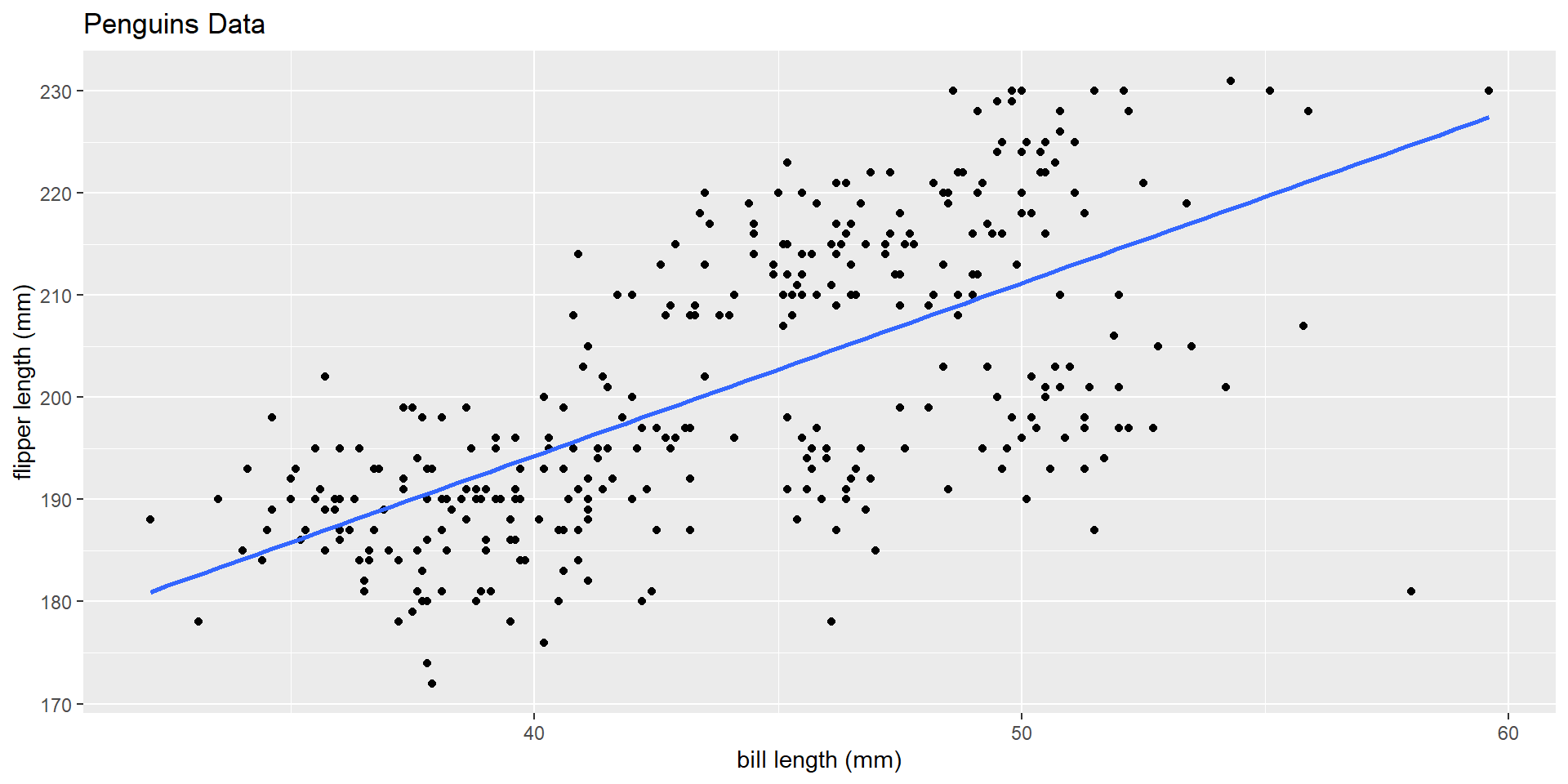
Last week, we talked at length about how these regression lines are fit:
Minimize the residual sums of squares: \(\sum (y_i - \hat{y_i})^2\)
This is true for both simple and multiple linear regression.
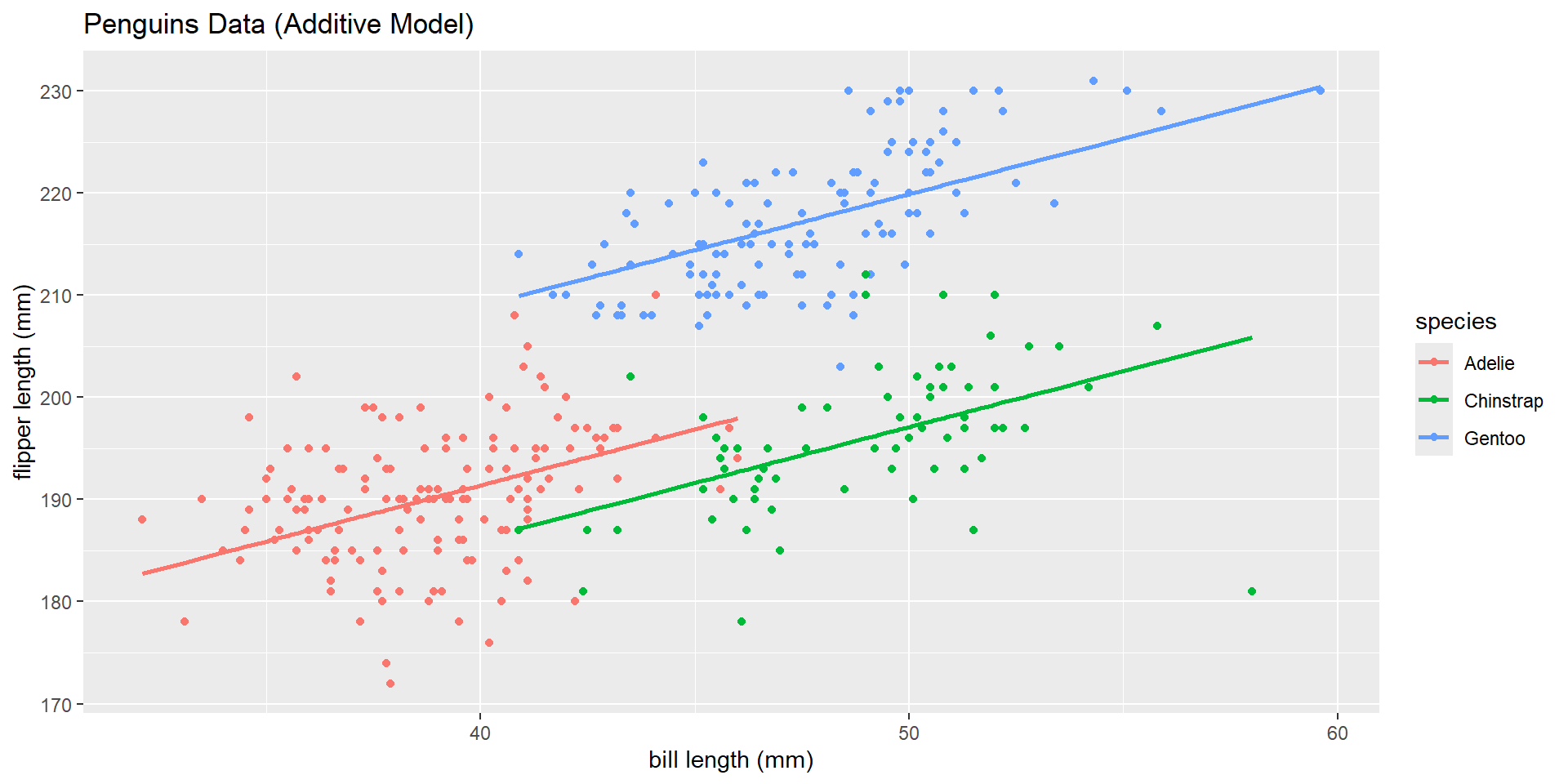
Visually that means…
Simple linear regression

Multiple linear regression

Why this matters?
The takeaway is that our model estimates are dependent on everything in our model. That is, the slope coefficient for bill length (mm) is not the same in SLR, as it is in MLR when we added species!
SLR Output
Call:
lm(formula = flipper_length_mm ~ bill_length_mm, data = penguins)

Residuals:
    Min      1Q  Median      3Q     Max
-43.413  -7.837   0.652   8.360  21.321

Coefficients:
               Estimate Std. Error t value Pr(>|t|)
(Intercept)    127.3304     4.7291   26.93   <2e-16 ***
bill_length_mm   1.6738     0.1067   15.69   <2e-16 ***
---
Signif. codes:  0 '***' 0.001 '**' 0.01 '*' 0.05 '.' 0.1 ' ' 1

Residual standard error: 10.63 on 331 degrees of freedom
Multiple R-squared:  0.4265,    Adjusted R-squared:  0.4248
F-statistic: 246.2 on 1 and 331 DF,  p-value: < 2.2e-16
MLR Output
Call:
lm(formula = flipper_length_mm ~ bill_length_mm + species, data = penguins)

Residuals:
     Min       1Q   Median       3Q      Max
-24.8669  -3.4617  -0.0765   3.7020  15.9944

Coefficients:
                 Estimate Std. Error t value Pr(>|t|)
(Intercept)      147.5633     4.2234  34.940  < 2e-16 ***
bill_length_mm     1.0957     0.1081  10.139  < 2e-16 ***
speciesChinstrap  -5.2470     1.3797  -3.803  0.00017 ***
speciesGentoo     17.5517     1.1883  14.771  < 2e-16 ***
---
Signif. codes:  0 '***' 0.001 '**' 0.01 '*' 0.05 '.' 0.1 ' ' 1

Residual standard error: 5.833 on 329 degrees of freedom
Multiple R-squared:  0.8283,    Adjusted R-squared:  0.8268
F-statistic: 529.2 on 3 and 329 DF,  p-value: < 2.2e-16
Takeaway
Model estimates change based on additional information you put in your model!
Questions?
Why not just fit the most complex model?
The parsimony principle for a statistical model states that: a simpler model with fewer parameters is favored over more complex models with more parameters, provided the models fit the data similarly well.
Why?
– More simple models are easier to interpret
– Can be more practically important
In short… keep it simple when you can…
In our context
If we are justified to fit an additive model with flipper length, bill length, and species… we should!
– Visual evidence (we will practice)
– Hypothesis testing
– Other model selection criteria (to compare models)
  > AIC
  > BIC
  > Adjusted R-Squared (we will cover)
Last time
Additive model
Call:
lm(formula = flipper_length_mm ~ bill_length_mm + species, data = penguins)

Residuals:
     Min       1Q   Median       3Q      Max
-24.8669  -3.4617  -0.0765   3.7020  15.9944

Coefficients:
                 Estimate Std. Error t value Pr(>|t|)
(Intercept)      147.5633     4.2234  34.940  < 2e-16 ***
bill_length_mm     1.0957     0.1081  10.139  < 2e-16 ***
speciesChinstrap  -5.2470     1.3797  -3.803  0.00017 ***
speciesGentoo     17.5517     1.1883  14.771  < 2e-16 ***
---
Signif. codes:  0 '***' 0.001 '**' 0.01 '*' 0.05 '.' 0.1 ' ' 1

Residual standard error: 5.833 on 329 degrees of freedom
Multiple R-squared:  0.8283,    Adjusted R-squared:  0.8268
F-statistic: 529.2 on 3 and 329 DF,  p-value: < 2.2e-16
Model Output
How can we simplify our model output to represent each of our three lines?
\(\widehat{\text{flipper length}} = 147.563 + 1.10*\text{bill length}\) \(- 5.25*\text{Chinstrap} + 17.55*\text{Gentoo}\)
\[\begin{cases} 1 & \text{if Chinstrap level}\\ 0 & \text{else} \end{cases}\] \[\begin{cases} 1 & \text{if Gentoo level}\\ 0 & \text{else} \end{cases}\]Visual

AE
Model Output
How can we simplify our model output to represent each of our three lines?
\(\widehat{\text{flipper length}} = 158.50 + 0.81*\text{bill length}\) \(- 11.87*\text{Chinstrap} + -8.26*\text{Gentoo} +\) \(0.19*\text{bill length}*\text{Gentoo} + 0.59*\text{bill length}*\text{Chinstrap}\)
\[\begin{cases} 1 & \text{if Chinstrap level}\\ 0 & \text{else} \end{cases}\] \[\begin{cases} 1 & \text{if Gentoo level}\\ 0 & \text{else} \end{cases}\]