# A tibble: 4 × 3
# Groups: supp [2]
supp measurement count
<fct> <chr> <int>
1 OJ High 23
2 OJ Low 7
3 VC High 18
4 VC Low 12Anova
Lecture: Not Sure
NC State University
ST 511 - Fall 2024
2024-10-21
Checklist
– Keep up with Slack
– Quiz Wednesday (due Sunday)
– HW-3 Friday (due Friday)
– Statistics experience (released Wednesday; due end of semester)
Announcements
– HW-2 is graded (re-grade requests back to TAs due by Friday at 5:00pm)
Announcements
– Exam-1 in-class is graded (released this afternoon)
> I'm going to post detailed solutions. Don't save and cycle them...
> If you have questions, please feel free to visit my office hours/email and I'll be happy to chat about it
Announcements
Class average ~ 71% (max ~ 99%); Exam-corrections
> There will be an "Optional" section on HW-3 that has questions around key concepts from exam-1
> Questions will be very similar
> Can earn 6 points back towards exam-1 in class (~7%)
> You can not earn more than a 100%
Reminder that if you filled out the survey (or do the optional assignment), your entire exam-1 grade gets scaled by 4%.
Your exam-1 total grade is the average between your in-class and take-home
Warm-up: exam-review
The response is the length of odontoblasts (cells responsible for tooth growth) in 60 guinea pigs. This is measured as “High” if the length of odontoblasts was larger than 10mm, and “Low” if the growth was 10mm or less. Each animal received doses of vitamin C either through a vitamin C supplement or by drinking orange juice, which has vitamin C in it.
We are interested in testing if the way the vitamin C was administered is independent from the odontoblasts length. You are researching if the orange juice (OJ) group produces more “High” measurements than the supplement group (VC). You can consider a “success” as a “High” measurement. Use the order of subtraction OJ - VC.
Warm-up: exam-review
We ask the questions:
– How many variable(s)?
– What type are they?
– If there are two, what is our explanatory? What is our response?
Warm-up: exam-review
The response is the length of odontoblasts (cells responsible for tooth growth) in 60 guinea pigs. This is measured as “High” if the length of odontoblasts was larger than 10mm, and “Low” if the growth was 10mm or less. Each animal received doses of vitamin C either through a vitamin C supplement or by drinking orange juice, which has vitamin C in it.
We are interested in testing if the way the vitamin C was administered is independent from the odontoblasts length. You are researching if the orange juice (OJ) group produces more “High” measurements than the supplement group (VC). You can consider a “success” as a “High” measurement. Use the order of subtraction OJ - VC.
Null and Alternative
\(H_o: \pi_\text{oj} - \pi_\text{vc} = 0\)
\(H_a: \pi_\text{oj} - \pi_\text{vc} > 0\)
Sample statistic
Statistic
\(\hat{p}_\text{oj} = \frac{23}{30}\)
\(\hat{p}_\text{vc} = \frac{18}{30}\)
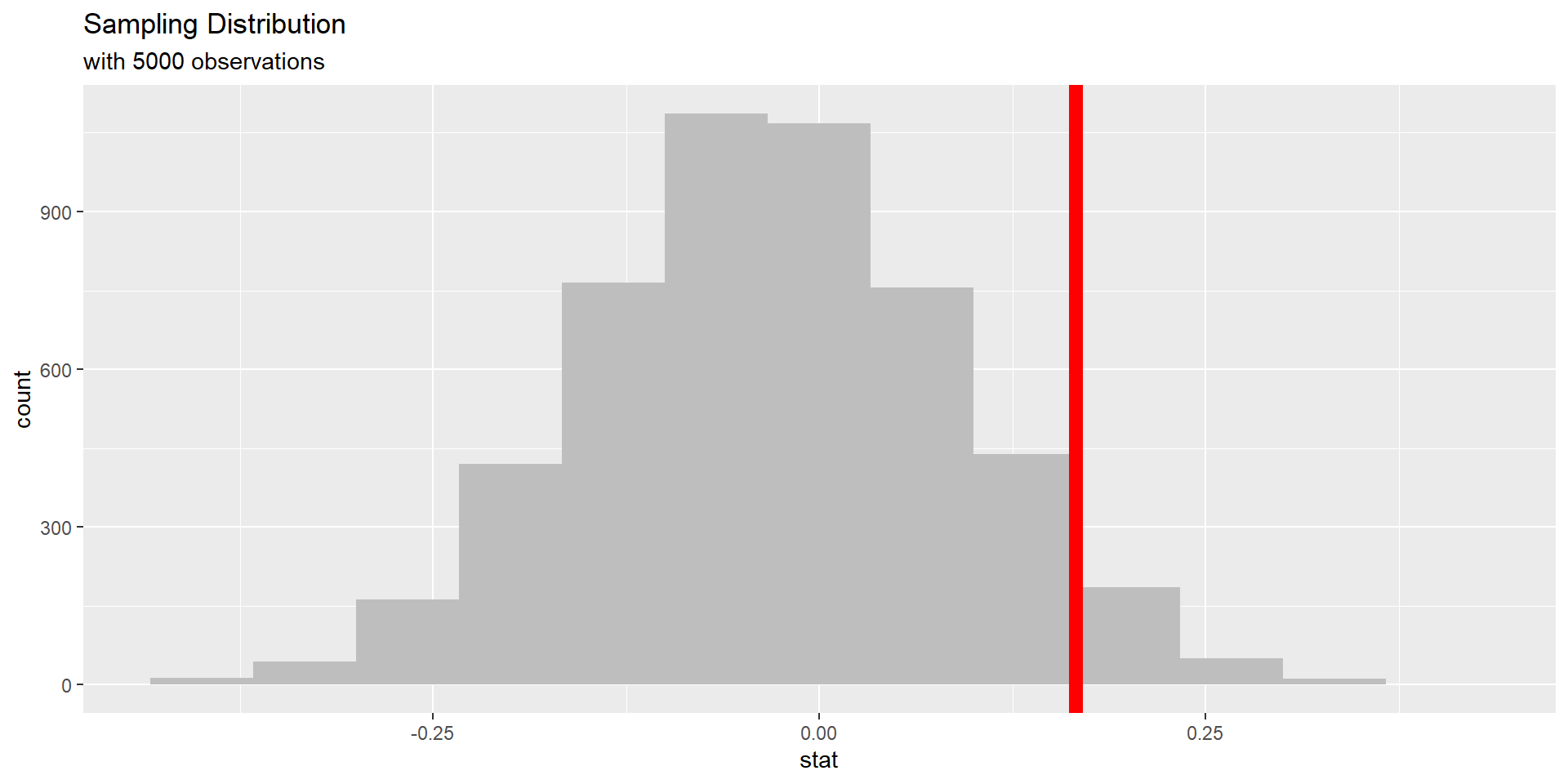
\(\frac{23}{30} - \frac{18}{30} = 0.167\)
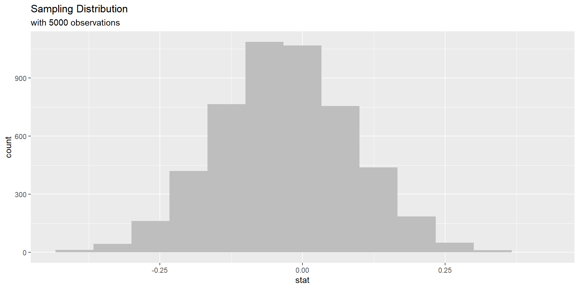
Simulated sampling distribution

In as much detail as possible, describe how one dot (observation) on this simulated sampling distribution under the assumption of the null hypothesis is created.
Simulation scheme
– shuffle all 60 observations together, because we assume independence
– shuffle observations (sample w/out replacement) into two new groups of size 30 each
– calculate each new sample proportion and subtract
p-values
The corresponding p-value for this test can be seen below.
# A tibble: 1 × 1
  p_value
    <dbl>
1   0.137
Describe how this p-value is calculated (interpret the p-value in the context of the problem).
p-values

p-values
p-value interpretation:
– probability of observing our statistic
– or something “more extreme” (larger)
– given the true proportion of high measurements is the same for the OJ and VC group
Questions
Last time
We were looking at the impact of species on bill length using the penguins data set. Why are we using Anova measures?
What is our null hypothesis?
What is our alternative hypothesis?
Null and alternative
\(H_o: \mu_g = \mu_c = \mu_a\)
\(H_a: \text{At least one population mean bill length is different}\)
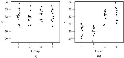
The Big Idea

The Big Idea

Anova
– What is our test statistic?
– What distribution does it follow?
F-distribution
with degrees of freedom of…
Numerator df = 3 - 1 = 2
We have 342 - 3 = 339
In R
# Compute the analysis of variance
res.aov <- aov(bill_length_mm ~ species, data = penguins)
# Summary of the analysis
summary(res.aov)
Df Sum Sq Mean Sq F value Pr(>F)
species 2 7194 3597 410.6 <2e-16 ***
Residuals 339 2970 9
---
Signif. codes: 0 '***' 0.001 '**' 0.01 '*' 0.05 '.' 0.1 ' ' 1
2 observations deleted due to missingnessDecision and conclusion
– Decision: We reject the null hypothesis…
– Conclusion: and have strong evidence to conclude that at least one population mean bill length is different
Which one(s)?
Tukeys HSD
The main idea of the hsd is to compute the honestly significant difference (hsd) between all pairwise comparisons
Why do we need to use this thing called Tukeys hsd? Why can’t we just conduct a bunch of individual hypothesis tests?
Type 1 error
\(\alpha\) is our significance level. It’s also our Type 1 error rate.
a Type 1 error is:
– rejecting the null hypothesis
– when the null hypothesis is actually true
Family-wise error rate
FWER = \(1 - (1-\alpha)^m\)
where m is the number of comparisons
Chocolate study

Pairwise comparisons
Commonly report confidence intervals to estimate which means are actually different (can also report p-values).
tukey’s hsd (technically Tukey-Kramer with unequal sample size)
\(\bar{x_1} - \bar{x_2} \pm \frac{q^*}{\sqrt{2}}* \sqrt{MSE*\frac{1}{n_j} + \frac{1}{n_j`}}\)
Where
– \(q^*\) is a value from the studentized range distribution
– (MSE) refers to the average of the squared differences between individual data points within each group and their respective group mean
\(q^*\) can be found using the qtukey function, or here
We are going to use a pre-packaged function in R to do the above calculations for us.
Results
  Tukey multiple comparisons of means
    95% family-wise confidence level

Fit: aov(formula = bill_length_mm ~ species, data = penguins)

$species
                      diff       lwr        upr     p adj
Chinstrap-Adelie 10.042433  9.024859 11.0600064 0.0000000
Gentoo-Adelie     8.713487  7.867194  9.5597807 0.0000000
Gentoo-Chinstrap -1.328945 -2.381868 -0.2760231 0.0088993
AE
Summary
Tukey’s Honest Significant Difference (HSD) test is a post hoc test commonly used to assess the significance of differences between pairs of group means. Tukey HSD is often a follow up to one-way ANOVA, when the F-test has revealed the existence of a significant difference between some of the tested groups.
