# A tibble: 1 × 3
  statistic chisq_df p_value
      <dbl>    <int>   <dbl>
1 0.0486 2 0.976Chi-square testing
Who’s counting?
NC State University
ST 511 - Fall 2024
Invalid Date
Checklist
– Keep up with Slack
– Quiz Wednesday (due Sunday)
– HW-3 due Sunday (Nov-3)
– Statistics experience (released; due end of semester on Gradescope)
– Optional assignment (released; due November 1st on Gradescope)
Announcements
HW-3 Exercise 1: Pick a test
I do not want you to write out an alternative hypothesis. You don’t have the information for this. This was corrected Saturday on both the HW + Starter.
Announcements
Exam-1 take-home grading
I write questions that try to get at your complete understanding of statistics
These questions are time consuming to grade
It’s also kind of your fault… because you write too much
Grades coming hopefully by the end of the week + key
Review of the process (Hypothesis Testing)
What variables are we working with
Regardless if you conducting your own research or working with others, it’s critical that we understand what the variable(s) are. This is justification for the type of methods we can use for analysis.
Scenario 1
The wait time for Starbucks at NC State seem to be increasing, and students are not happy…. To try and solve this issue, the manager bought a new coffee machine. They want to know if the new machine makes drinks faster than the old one. Over the course of 1-week, the time (in seconds) it takes for the coffee machines to make a drink were recorded across the old machine (machine A) and the new machine (machine B).
What are the variables?
What is the scenario?
What is the null hypothesis?
Scenario 1
time in seconds (quantitative response)
machine type (a or b; categorical explanatory)
\(Ho: \mu_a = \mu_b\)
Scenario 2
8.1% of middle and high school students reported current tobacco use in 2024. You are interested if middle and high school students in the State of North Carolina are less than the national percentage.
Scenario 2
Do you use tobacco? (Yes or no; categorical)
\(Ho: \pi = .081\)
We then collect data
and calculate our sample statistic
\(\bar{x}\)
\(\hat{p}\)
MSE and MST for anova
etc.
Simulation vs Theory Based
Simulation:
– Assume the null hypothesis to be true
– and after checking assumptions
– We use our data to simulate a sampling distribution of statistics under the assumption of the null hypothesis

Simulation vs Theory Based
Theory Based
– Assume the null hypothesis to be true
– and after checking assumptions
– We can standardize our statistic…
\[ \frac{stat - null}{SE} \]
so then it follows a distribution if the null hypothesis were really true (assume the null to be true)

New method (same process)
Sex vs Species
Suppose that we want to look at the relationship between sex and species. That is, we want to test if species of penguin is independent from sex. Let’s remind ourselves how many species there.
Type of test
Can we use difference in means?
Difference in proportions?
Chi-square test
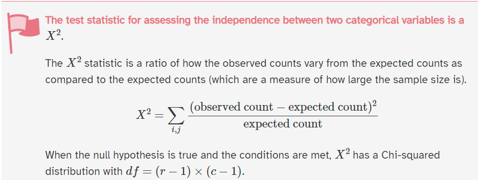
The big picture idea is to compare expected counts (under the assumption of the null hypothesis with observed counts. This is how we are going to calculate our test statistic.
Assumptions
Independence
Expected frequencies
Expected frequencies
The expected counts are not too low. The rule of thumb is that the expected values (not the observed counts!) should be greater than 5. If any of the expected values are below 5 the p-values generated by the test start to become less reliable.
We will check this when we make a table!
Chi-square test
The big picture idea is to compare expected counts (under the assumption of the null hypothesis with observed counts. This is how we are going to calculate our test statistic.
Null hypothesis
What is our null hypothesis?
What is our alternative hypothesis?
Null hypothesis
\(Ho\) Species has no impact on sex OR Species is completely independent from sex
\(Ha\) Species has some impact on sex OR Species is not independent from sex
Chi-square test
The big picture idea is to compare expected counts (under the assumption of the null hypothesis with observed counts. This is how we are going to calculate our test statistic.
– Null hypothesis ✔️
Expected counts
Expected counts
With a sample size of 333, what would we expect to see in this table under the assumption that species and sex are independent?
Table of EXPECTED counts
| Male | Female | Total | |
|---|---|---|---|
| Adelie | 146 | ||
| Chinstrap | 68 | ||
| Gentoo | 119 | ||
| Total | 168 | 165 | 333 |
Expected Formula

Expected Table
| Male | Female | Total | |
|---|---|---|---|
| Adelie | (146*168)/333 | 146 | |
| Chinstrap | (68*168)/333 | 68 | |
| Gentoo | (119*168)/333 | 119 | |
| Total | 168 | 165 | 333 |
Expected Table
| Male | Female | Total | |
|---|---|---|---|
| Adelie | 73.658 | 146 | |
| Chinstrap | 34.306 | 68 | |
| Gentoo | 60.036 | 119 | |
| Total | 168 | 165 | 333 |
If there is no difference between sex and species, we would expect to observe this values above from our sample.
Expected Table
| Male | Female | Total | |
|---|---|---|---|
| Adelie | 73.658 | 146 | |
| Chinstrap | 34.306 | 68 | |
| Gentoo | 60.036 | 119 | |
| Total | 168 | 165 | 333 |
Calculate the expected number of Female penguins for each of the three species
Expected Table
| Male | Female | Total | |
|---|---|---|---|
| Adelie | 73.658 | (146*165)/333 = 72.343 | 146 |
| Chinstrap | 34.306 | (68*165)/333 = 33.694 | 68 |
| Gentoo | 60.036 | (119*165)/333 = 58.964 | 119 |
| Total | 168 | 165 | 333 |
Are these all larger than 5?
Chi-square test
The big picture idea is to compare expected counts (under the assumption of the null hypothesis with observed counts. This is how we are going to calculate our test statistic.
– Null hypothesis ✔️
– Expected ✔️
– Observed counts
Observed
| Male | Female | Total | |
|---|---|---|---|
| Adelie | 73 | 73 | 147 |
| Chinstrap | 34 | 34 | 68 |
| Gentoo | 61 | 58 | 119 |
| Total | 168 | 165 | 333 |
Observed vs Expected
Expected values are in ( )
| Male | Female | Total | |
|---|---|---|---|
| Adelie | 73 (73.658) | 73 (72.342) | 146 |
| Chinstrap | 34 (34.306) | 34 (33.694) | 68 |
| Gentoo | 61 (60.036) | 58 (58.964) | 119 |
| Total | 168 | 165 | 333 |
What do we think? Without doing a formal test, do you think we will reject or fail to reject the null hypothesis? Why?
Chi-square test
The big picture idea is to compare expected counts (under the assumption of the null hypothesis with observed counts. This is how we are going to calculate our test statistic.
– Null hypothesis ✔️
– Expected ✔️
– Observed counts ✔️
Let’s perform the test

where r is the number of groups for one variable (rows) and c is the number of groups for the second variable (columns)
Chi-sqaure
– The shape of the chi-square distribution curve depends on the degrees of freedom
– Test statistic can not be negative
– The chi-square distribution curve is skewed to the right, and the chi-square test is always right-tailed
– A chi-square test cannot have a directional hypothesis. A chi-square value can only indicate that a relationship exists between two variables, not what the relationship is.
Questions
In R
We are going to use the chisq_test() function in the infer package
syntax: data, y, x
“By hand”
Why do we have a lower.tail argument? Not sure…. make sure it’s false.
Let’s talk about it
Decision?
Conclusion?
Let’s talk about it
Fail to reject the null hypothesis
Weak evidence to conclude that species has an impact on sex
Summary
– Chi-square testing is used when we want to test for independence when we have a categorical variable with > 2 levels
– Always right tailed test
– df of (r-1)*(c-1)
