Connecting Packaged R Code with Concepts + Intro to regression
Lecture: Not Sure
NC State University
ST 511 - Fall 2024
2024-10-30
Download today’s AE oct-30 from Moodle. We are going to learn a new distribution!
…not really, but you still need to download the AE for today
Checklist
– Keep up with Slack
– Upload today’s AE. We will be using this to start class
– Homework 3 (including exam corrections) due Sunday (11:59pm)
– Quiz Wednesday (due Sunday)
– Statistics experience (released; due end of semester on Gradescope)
– Optional assignment (released; due November 1st on Gradescope)
Learning objectives
– Review some common “pre-packaged” functions you will commonly see used to analyze data
– Understand what the output means / describe the output
– What is regression?
– Understand how to summarize two quantitative variables
The AE
Before we get into the AE, I want to make it clear that this AE is designed for us to explore and understand common data analysis functions in R, and make connections to what we’ve learned in class.
A rigorous analysis would include:
– Exploratory data analysis
– Checking assumptions
– Writing decisions + conclusions
– ect.
I want you all to be familiar with these functions in R, just in case you come across/need them in your future work.
AE 10-30
t-test
syntax for t.test
t.test(y ~ x = NULL, alternative = c("two.sided", "less", "greater"), mu = 0, paired = FALSE, var.equal = FALSE, conf.level = 0.95, …)
Can just use y for single mean test!
t-test
Assumptions
– Independence
– Normality
– Note: We can also check for constant variance. If we find this to be true, we can use a different type of SE.
t-test
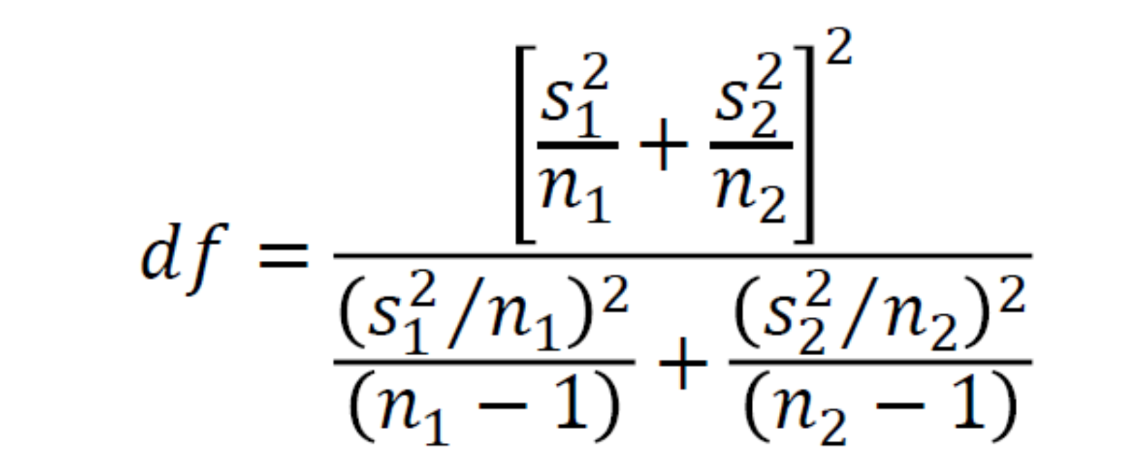
One-sided confidence interval
You do not need to know this for this course.
“In a one-sided confidence interval, we’re trying to find a single number a such that we’re 95% confident that the true mean is greater than a (or less than a if you set one.sided=”less”)“.
t-test
\[ t = \frac{\bar{x_1} - \bar{x_2} - 0}{\sqrt{\frac{s_1^2}{n1} + \frac{s_2^2}{n2}}} \]
t-test
\[ t = \frac{5.78 - 9.22 - 0}{\sqrt{\frac{2.88^2}{10} + \frac{3.48^2}{10}}} = -2.41 \]
Anova
Assumptions
– Independence
– Normality
– Constant Variance
Anova
syntax: y ~ x, data =
Anova
syntax: y ~ x, data =
Chi-sq
Assumptions
– Independence
– Expected counts larger than 5
Chi-sq
syntax: chisq_test(data, y ~ x)
Chi-sq
syntax: chisq_test(survey, W.Hnd ~ Clap)
Regression
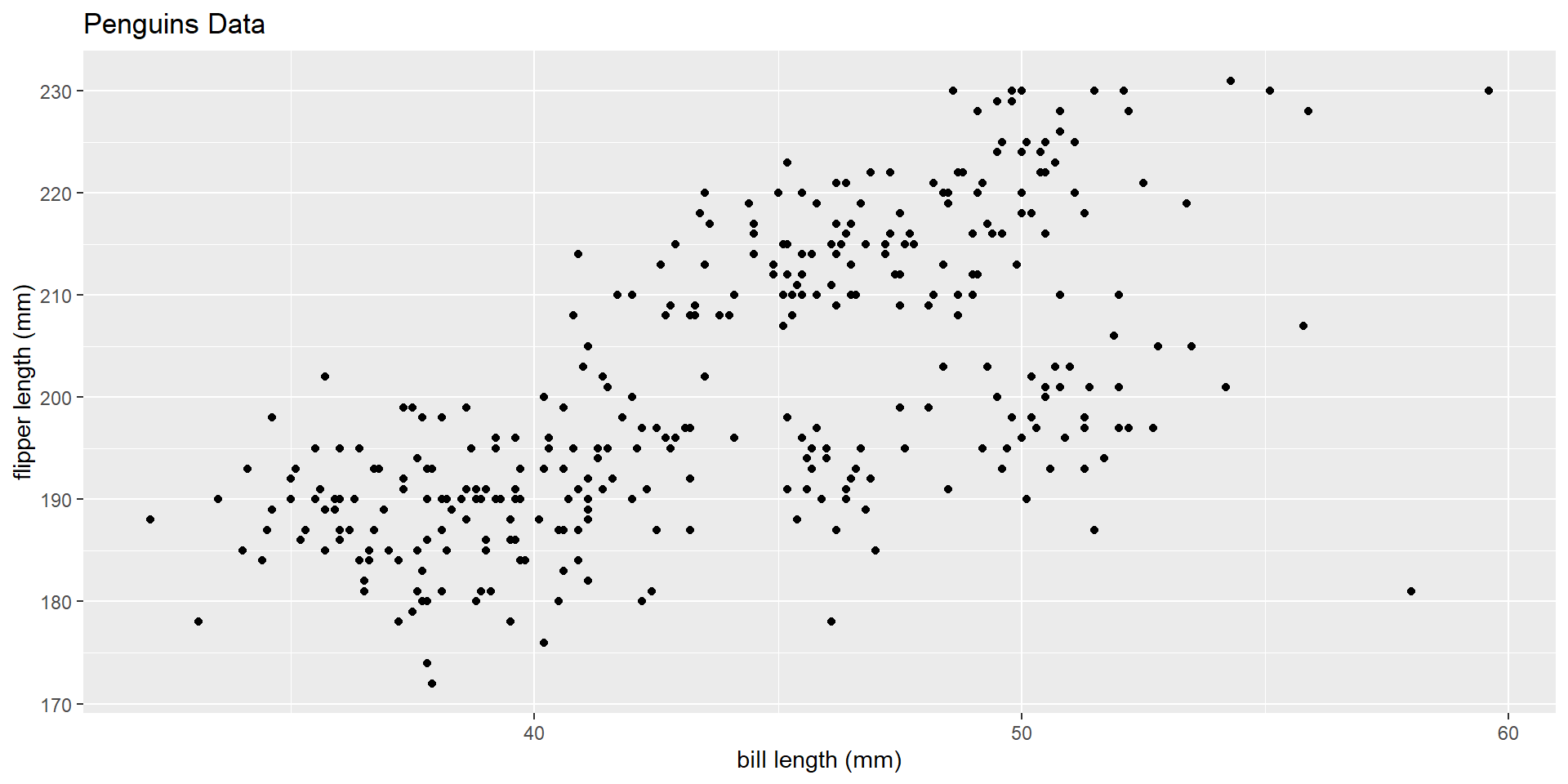
Suppose now I wanted to investigate the relationship between bill length and flipper length.
– Can I analyze these data using difference in means?
– Difference in proportions?
What plot could we use to look at these data?
Plot the data
How can we summarize these data?
Summary statistics
– correlation (r)
– slope + intercept (fit a line)
Correlation
– Is bounded between [-1, 1]
– Measures the strength + direction of a linear relationship
What do I mean by linear relationship?
What do I mean by strength?
What do I mean by direction?

Guessing Game
Fit a line
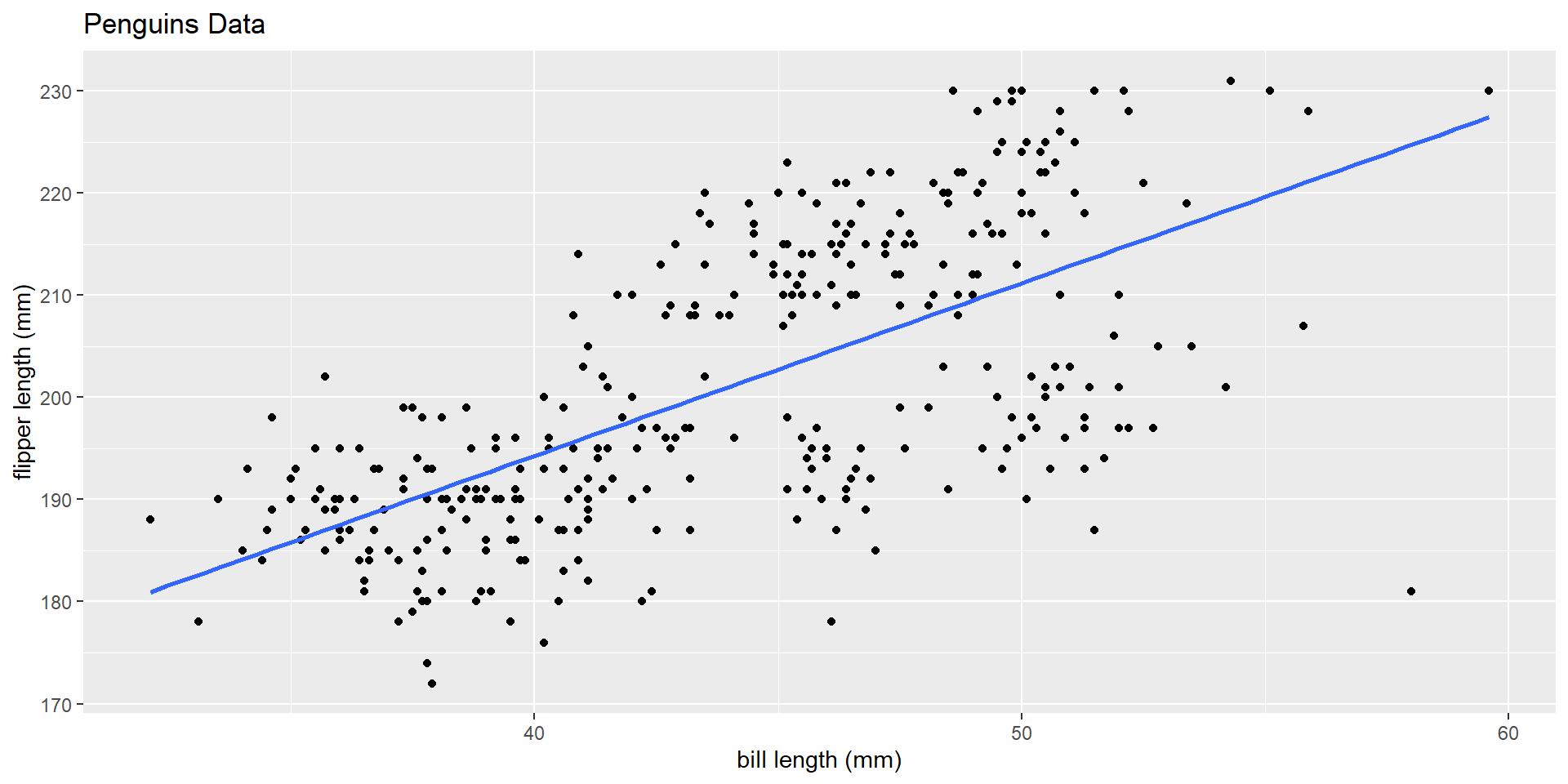
How do we suppose that this line was fit?
Residual
\(e_i = y - \hat{y}\)
where y is an observed value, and \(\hat{y}\) is the predicted value based on the line!
Residual
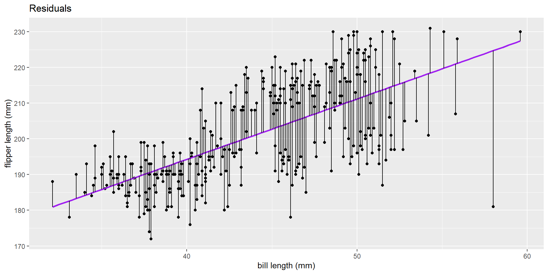
Why do you suppose we fit a line?
Why do you suppose we fit a line?
– Prediction
– Interpretation
– Hypothesis testing to test for a relationship
The equation
Have you heard of \(y = mx + b\) ?
The equation
Let me introduce you to
\(\hat{y} = \hat{\beta_o} + \hat{\beta_1}*x\)
The equation
\(\hat{y}\) = predicted value of y
\(\hat{\beta_o}\) = estimated intercept
\(\hat{\beta_1}\) = estimated slope
\(x\) = explanatory variable
In-R
Call:
lm(formula = flipper_length_mm ~ bill_length_mm, data = penguins)

Residuals:
    Min      1Q  Median      3Q     Max
-43.708  -7.896   0.664   8.650  21.179

Coefficients:
               Estimate Std. Error t value Pr(>|t|)
(Intercept)    126.6844     4.6651   27.16   <2e-16 ***
bill_length_mm   1.6901     0.1054   16.03   <2e-16 ***
---
Signif. codes:  0 '***' 0.001 '**' 0.01 '*' 0.05 '.' 0.1 ' ' 1

Residual standard error: 10.63 on 340 degrees of freedom
  (2 observations deleted due to missingness)
Multiple R-squared:  0.4306,    Adjusted R-squared:  0.4289
F-statistic: 257.1 on 1 and 340 DF,  p-value: < 2.2e-16