weight feed
Min. :108.0 casein :12
1st Qu.:204.5 horsebean:10
Median :258.0 linseed :12
Mean :261.3 meatmeal :11
3rd Qu.:323.5 soybean :14
Max. :423.0 sunflower:12 Exam-Review
Last one!
NC State University
ST 511 - Fall 2024
2024-12-02
Checklist
– Keep up with Slack
– HW 4 published over weekend (re-grade are due by Tuesday at 5:00pm)
– HW 5 goal to be published Dec2/3 (Key is already posted)
– HW 6 goal to be published Dec 6 (Key is already posted)
– Don’t forget about the statistics experience (Due Dec 6th)
Announcements
Office hours:
– Will be holding additional office hours this week (See Slack)
– Will not be holding office hours during finals week (do not want to give advantage to one section over the other)
Announcements
Location: This room
Section-1 (3:00pm class) is on Wed Dec 11 from 3:30 - 6:00pm
Section-2 (11:45pm class) is on Mon Dec 9 from 12:00 - 2:30pm
Announcements
Final Exam Note Sheet:
– You are allowed one front+back note sheet on the final exam
  > It must be hand-written
  > I will also provide you a formula sheet + get it posted to our website ~ 1 week (if not sooner) before the final exam
– I suggest writing things such as..
  > General interpretations (slope coefficient; p-value; etc)
  > "Conversational" questions to help discover answers (what is my explanatory variable; is it categorical or quantitative; if categorical, how many levels?)
Questions about the Final
Question 1
An experiment was conducted to measure and compare the effectiveness of various feed supplements on the growth rate of chickens.
– What types of variables are we working with?
– Which is the explanatory? Which is the response?
Answer
– What types of variables are we working with?
weight (quantitative response) measured in grams
feed (categorical explanatory) with 6 levels
What type of test should we use to analyze these data?
Anova
What is the null and alternative hypothesis to analyze the relationship between feed and weight?
Null and Alternative
\(Ho: \mu_c = \mu_h = \mu_l = \mu_m = \mu_\text{soy} = \mu_\text{sun}\)
Ha: at least one population mean weight is different across the six different feeds
Anova
In order to trust our results, we need to check assumptions. What are they?
Assumptions
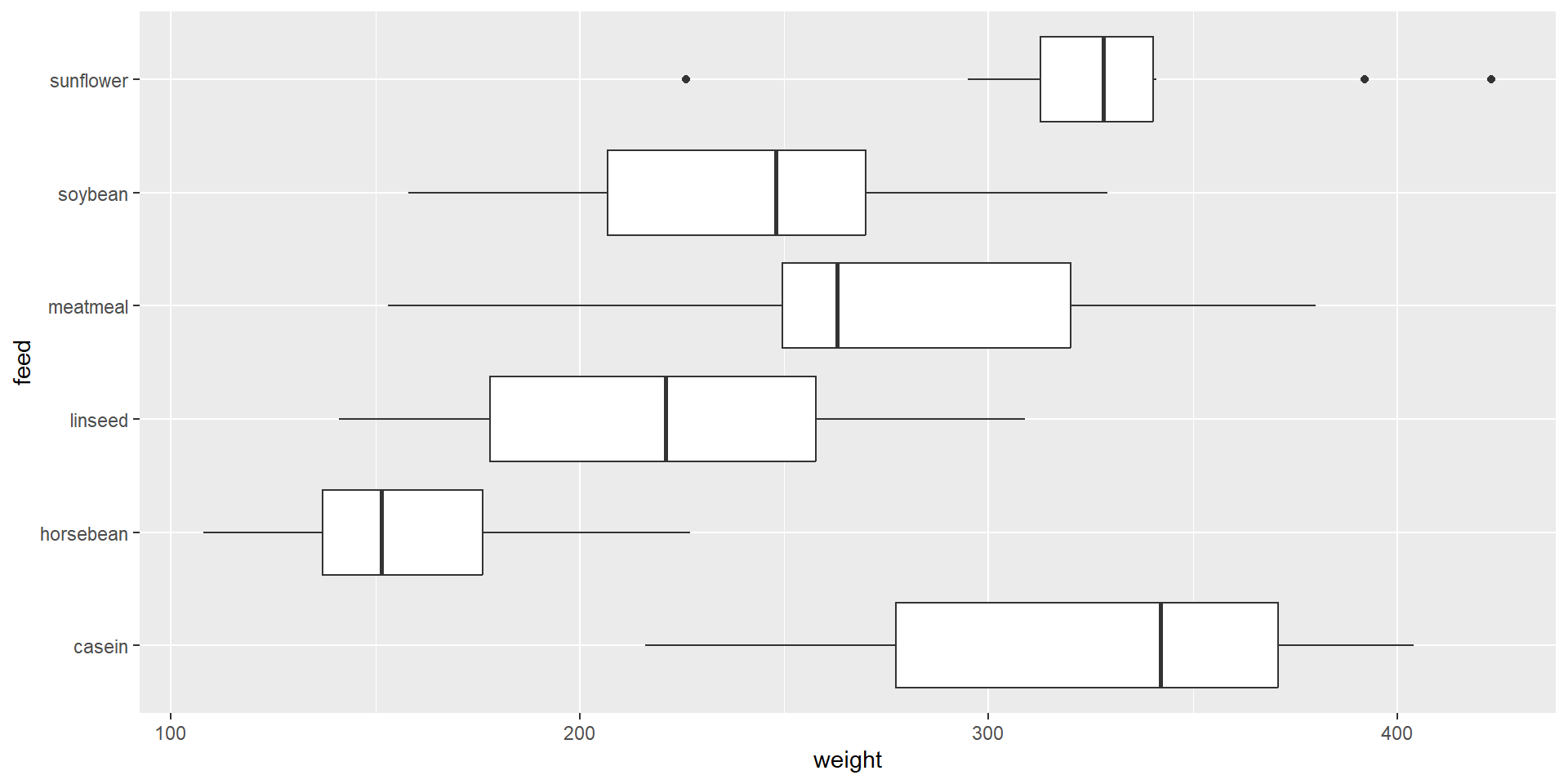
Assumptions
# A tibble: 6 × 2
  feed         sd
  <fct>     <dbl>
1 casein     64.4
2 horsebean  38.6
3 linseed    52.2
4 meatmeal   64.9
5 soybean    54.1
6 sunflower  48.8
Assumptions (not on exam)
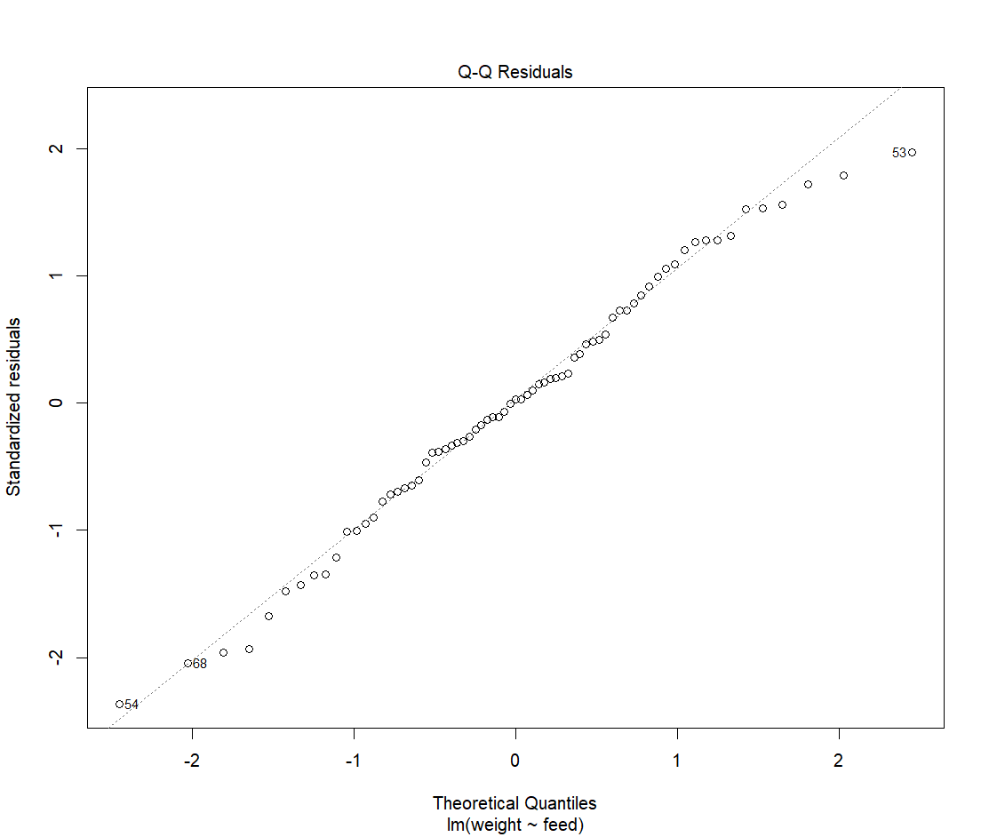
If standardized residuals mostly fall on the line, not enough evidence to reject the normality assumption
Anova
            Df Sum Sq Mean Sq F value   Pr(>F)
feed         5 231129   46226   15.37 5.94e-10 ***
Residuals   65 195556    3009
---
Signif. codes:  0 '***' 0.001 '**' 0.01 '*' 0.05 '.' 0.1 ' ' 1
– Where do the DF come from?
– What do the Sum Sq represent?
– How are Mean Sq calculated?
– Write an appropriate decision and conclusion in the context of the problem
Question 2
For this question, we are going to use the survey data set. This data frame contains the responses of 237 Statistics I students at the University of Adelaide to a number of questions.
We are interested in comparing the relationship between the span (measured in centimeters) of a student’s writing hand, and the span of their non-writing hand. That is, can we use the span of a student’s non-writing hand to predict the span of their writing hand?
– What are the variables? Type? Explanatory vs response?
– What method could we use to investigate this relationship?
Answers
– What are the variables? Type? Explanatory vs response?
Span of writing hand (quantitative response); Span of non-writing hand (quantitative explanatory)
Simple linear regression!
SLR
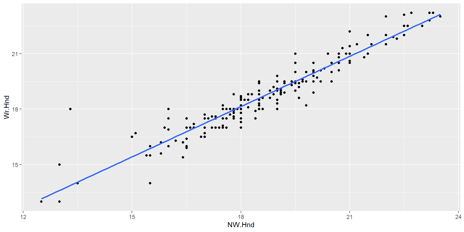
– How was this line fit?
– Describe the relationship between our 2 variables (strength + direction)
– Guess the correlation coefficient!
Answers
– How was this line fit?
Line of best fit = minimizing the residual sums of squares
– Describe the relationship between our 2 variables (strength + direction)
Strong positive relationship
– Guess the correlation coefficient!
Close to 1 (.7-1). Strong positive linear relationship between x and y
Extension
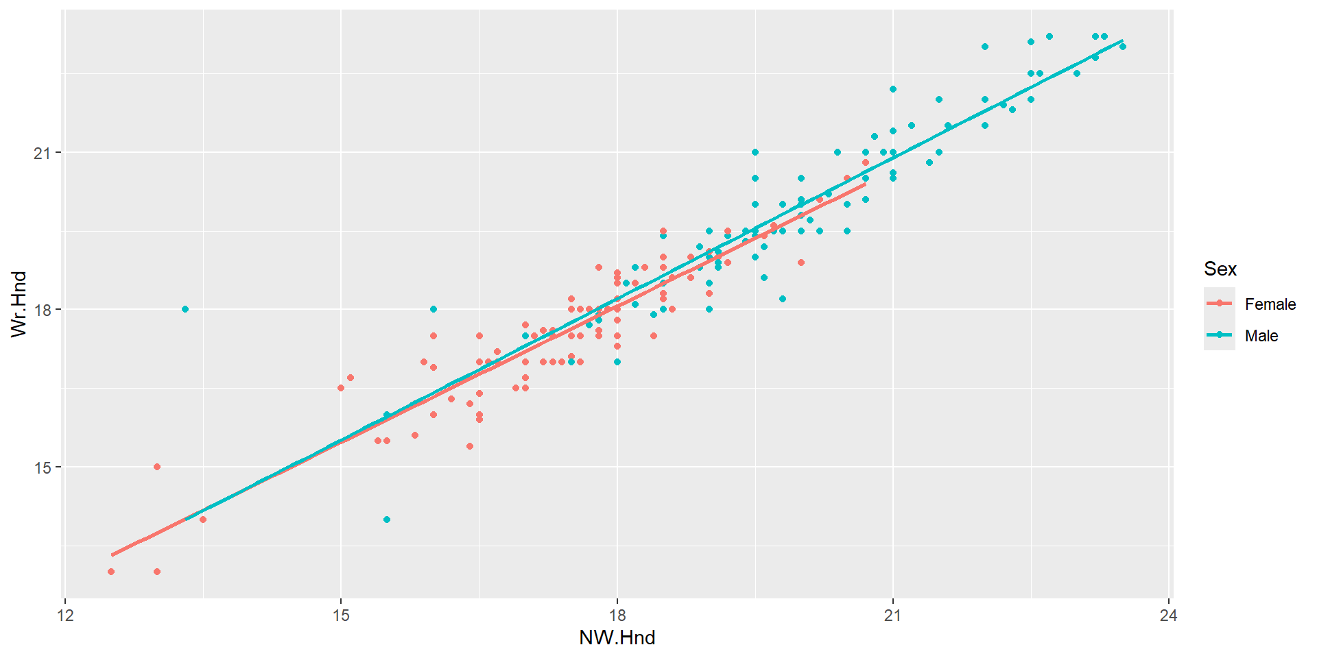
What if we wanted to compare this relationship by sex?
Based on the plot below, would you suggest fitting an additive model or an interaction model? Why?
What’s the difference between the two models?
Model
Write out the model in proper notation using the output below
Call:
lm(formula = Wr.Hnd ~ NW.Hnd + Sex, data = survey)

Residuals:
    Min      1Q  Median      3Q     Max
-2.0189 -0.3182 -0.0524  0.3077  3.9245

Coefficients:
            Estimate Std. Error t value Pr(>|t|)
(Intercept)  2.17507    0.42408   5.129 6.15e-07 ***
NW.Hnd       0.88336    0.02409  36.670  < 2e-16 ***
SexMale      0.15170    0.09476   1.601    0.111
---
Signif. codes:  0 '***' 0.001 '**' 0.01 '*' 0.05 '.' 0.1 ' ' 1

Residual standard error: 0.5948 on 232 degrees of freedom
  (2 observations deleted due to missingness)
Multiple R-squared:  0.9009,    Adjusted R-squared:  0.9001
F-statistic:  1055 on 2 and 232 DF,  p-value: < 2.2e-16
Model
\(\widehat{Wr.Hnd} = 2.175 + .883*NW.Hnd + .151*Male\)
\[\begin{cases} 1 & \text{if Male level}\\ 0 & \text{else} \end{cases}\]What do these three values represent?
Question 3
For this question, we are going to use the same survey data set. Now, we are interested in predicting the probability of one’s Sex, based on which arm is on top when a student folds their hands.
     Sex           Fold
 Female:118   L on R : 98
 Male  :118   Neither: 18
              R on L :120
– What is our response variable? Explanatory variable(s)?
– Types of variables?
– Method we can use to analyze these data?
Answers
– What is our response variable? Explanatory variable?
Sex is the response; Fold is the explanatory
– Types of variables?
Sex is categorical; Fold is categorical
– Method we can use to analyze these data?
Logistic regression Note, we could use a chi-square test if our research question was interested in independence between our variables.
Model
Note: We can consider “success” as Male.
               Estimate Std. Error    z value  Pr(>|z|)
(Intercept)  0.04082199  0.2020726  0.2020165 0.8399038
FoldNeither  0.65232519  0.5392896  1.2096010 0.2264320
FoldR on L  -0.17435339  0.2726087 -0.6395739 0.5224496
Now, write out the model in proper notation using the summary output above.
Model
\(\widehat{ln\frac{p}{1-p}} = 0.048 + .652*Neither - .174*RonL\)
\[\begin{cases} 1 & \text{if Neither level}\\ 0 & \text{else} \end{cases}\] \[\begin{cases} 1 & \text{if R on L level}\\ 0 & \text{else} \end{cases}\]– Calculate the estimated log odds of Neither
– Calculate the estimated probability of being a male given a student puts neither hand on top when they fold
Log odds
\(\widehat{ln\frac{p}{1-p}} = 0.048 + .652*1 - .174*0\)
\(\widehat{ln\frac{p}{1-p}} = 0.048 + .652*1\)
\(\widehat{ln\frac{p}{1-p}} = 0.048 + .652*1\)
\(\widehat{ln\frac{p}{1-p}} = 0.70\)
Probability
\(\hat{p} = \frac{e^{\widehat{\beta_o} + \widehat{\beta_1}\text{Neither}}}{1 + e^{\widehat{\beta_o} + \widehat{\beta_1}\text{Neither}}}\)
\(\hat{p} = \frac{e^.70}{1 + e^.70}\) = .668
Question 4
Data from a case-control study of esophageal cancer in Ille-et-Vilaine, France. Below are the data. We are initially interested in the relationship between a person’s age, and their tobacco consumption. More specifically, we want to know if age is independent from tobacco use.
   agegp         tobgp
 25-34:15   0-9g/day:24
 35-44:15   10-19   :24
 45-54:16   20-29   :20
 55-64:16   30+     :20
 65-74:15
 75+  :11
What are the variable types?
What method should we use to analyze these data?
Chi-square
Because our variables are categorical, with > 2 levels, we are going to conduct a chi-square test of independence.
What are the assumptions?
Assumptions
– Independence
– Expected counts > 5
Null and Alternative
– What is the null and alternative hypothesis for this test?
– What is the statistic?
– What distribution does the statistic follow under the assumption of the null?
– What are the degrees of freedom with this distribution?
Answers
– What is the null and alternative hypothesis for this test?
\(Ho: \text{Age and tobacco use are independent}\) \(Ha: \text{Age and tobacco use are dependent}\)
– What is the statistic?
\(\chi^2\)
– What distribution does the statistic follow under the assumption of the null?
chi-square distribution
– What are the degrees of freedom with this distribution?
(6-1)*(4-1) = 15
Output
    Pearson's Chi-squared test

data:  esoph_expand$agegp and esoph_expand$tobgp
X-squared = 27.499, df = 15, p-value = 0.02492
Can we trust it?
                  esoph_expand$tobgp
esoph_expand$agegp  0-9g/day    10-19    20-29       30+
             25-34  66.32903 26.41290 14.69032  7.567742
             35-44 109.58710 43.63871 24.27097 12.503226
             45-54  96.32129 38.35613 21.33290 10.989677
             55-64  95.74452 38.12645 21.20516 10.923871
             65-74  61.13806 24.34581 13.54065  6.975484
             75+    17.88000  7.12000  3.96000  2.040000