Additive + Interaction Models: Solutions
Load packages and data
Today
By the end of today you will…
- be able to build, fit and interpret linear models with \(>1\) predictor
- think critically about r-squared as a model selection tool
- use adjusted r-squared to compare models
Interaction model
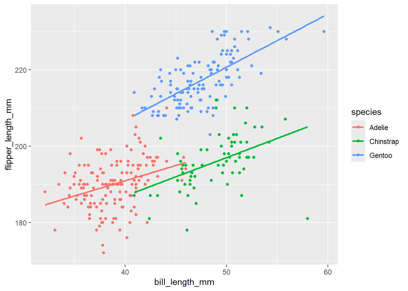
First, let’s visualize
penguins |>
  ggplot(
    aes(x = bill_length_mm, y = flipper_length_mm, color = species)
  ) +
  geom_point() +
  geom_smooth(method = "lm", se = F)
`geom_smooth()` using formula = 'y ~ x'Warning: Removed 2 rows containing non-finite outside the scale range
(`stat_smooth()`).Warning: Removed 2 rows containing missing values or values outside the scale range
(`geom_point()`).
Now, let’s fit an interaction model to get the estimates associated with the plot above. Name this model_int. Provide the summary output.
Call:
lm(formula = flipper_length_mm ~ bill_length_mm * species, data = penguins)

Residuals:
     Min       1Q   Median       3Q      Max
-24.0561  -3.3195  -0.1806   3.5830  16.4397

Coefficients:
                                Estimate Std. Error t value Pr(>|t|)
(Intercept)                     158.9244     6.9039  23.020  < 2e-16 ***
bill_length_mm                    0.7999     0.1776   4.505 9.17e-06 ***
speciesChinstrap                -12.2886    12.4595  -0.986   0.3247
speciesGentoo                    -7.8284    10.6428  -0.736   0.4625
bill_length_mm:speciesChinstrap   0.2073     0.2765   0.750   0.4538
bill_length_mm:speciesGentoo      0.5913     0.2459   2.405   0.0167 *
---
Signif. codes:  0 '***' 0.001 '**' 0.01 '*' 0.05 '.' 0.1 ' ' 1

Residual standard error: 5.792 on 336 degrees of freedom
  (2 observations deleted due to missingness)
Multiple R-squared:  0.8328,    Adjusted R-squared:  0.8303
F-statistic: 334.8 on 5 and 336 DF,  p-value: < 2.2e-16
And just like before, we can make predictions!
predict(model_int, data.frame(bill_length_mm = 40, species = "Adelie")) 1
190.9204 Now, simplify our model for just the Chinstrap penguins, showing how both the slope and intercept change from the baseline in this interaction model.
See demo on doc-cam: take notes here
Model selection
Let’s talk more about r-squared
As a reminder, \(R^2\) is defined as the amount of variability in our response (y) that is explained by our model with x explanatory variable(s)
Demo
set.seed(12345)
random_peng <- rbeta(nrow(penguins), 20, 10) # make 100 random numbers

penguins_fake <- cbind(penguins, random_peng) # add that variable to the data

####### models + r.squared value

slr_model <- lm(flipper_length_mm ~ bill_length_mm, data = penguins_fake)
summary(slr_model)$r.squared # slr model
[1] 0.430574add_model <- lm(flipper_length_mm ~ bill_length_mm + species, data = penguins_fake)
summary(add_model)$r.squared # additive model[1] 0.8298693summary(model_int)$r.squared # interaction model[1] 0.8328305nonsense_model <- lm(flipper_length_mm ~ bill_length_mm*species*random_peng, data = penguins_fake )
summary(nonsense_model)$r.squared #interaction model with a literal random variable[1] 0.8441509Can we use r-squared for model selection? Why or why not?
We can not use R^2 for model selection. This value always increases as your model gets more complicated, even if you add variables that do not make sense
Adjusted r.squared
summary(slr_model)$adj.r.squared # slr model[1] 0.4288992summary(add_model)$adj.r.squared # additive model[1] 0.8283592summary(model_int)$adj.r.squared # interaction model[1] 0.8303428summary(nonsense_model)$adj.r.squared # nonsense model[1] 0.8389559Takeaway: Our interaction model with bill length and species provides us with the best overall model fit, after accounting for the number of parameters in the model.
