Estimating penguins bill length (mm)

Using simulation

The following code can be used to calculated a confidence interval using simulation techniques. This is in the context of class for October 2nd.

Packages

library(tidyverse)

── Attaching core tidyverse packages ──────────────────────── tidyverse 2.0.0 ──
✔ dplyr     1.1.4     ✔ readr     2.1.5
✔ forcats   1.0.0     ✔ stringr   1.5.1
✔ ggplot2   3.5.1     ✔ tibble    3.2.1
✔ lubridate 1.9.3     ✔ tidyr     1.3.1
✔ purrr     1.0.2     
── Conflicts ────────────────────────────────────────── tidyverse_conflicts() ──
✖ dplyr::filter() masks stats::filter()
✖ dplyr::lag()    masks stats::lag()
ℹ Use the conflicted package (<http://conflicted.r-lib.org/>) to force all conflicts to become errors

library(tidymodels)

── Attaching packages ────────────────────────────────────── tidymodels 1.2.0 ──
✔ broom        1.0.6     ✔ rsample      1.2.1
✔ dials        1.3.0     ✔ tune         1.2.1
✔ infer        1.0.7     ✔ workflows    1.1.4
✔ modeldata    1.4.0     ✔ workflowsets 1.1.0
✔ parsnip      1.2.1     ✔ yardstick    1.3.1
✔ recipes      1.1.0     
── Conflicts ───────────────────────────────────────── tidymodels_conflicts() ──
✖ scales::discard() masks purrr::discard()
✖ dplyr::filter()   masks stats::filter()
✖ recipes::fixed()  masks stringr::fixed()
✖ dplyr::lag()      masks stats::lag()
✖ yardstick::spec() masks readr::spec()
✖ recipes::step()   masks stats::step()
• Search for functions across packages at https://www.tidymodels.org/find/

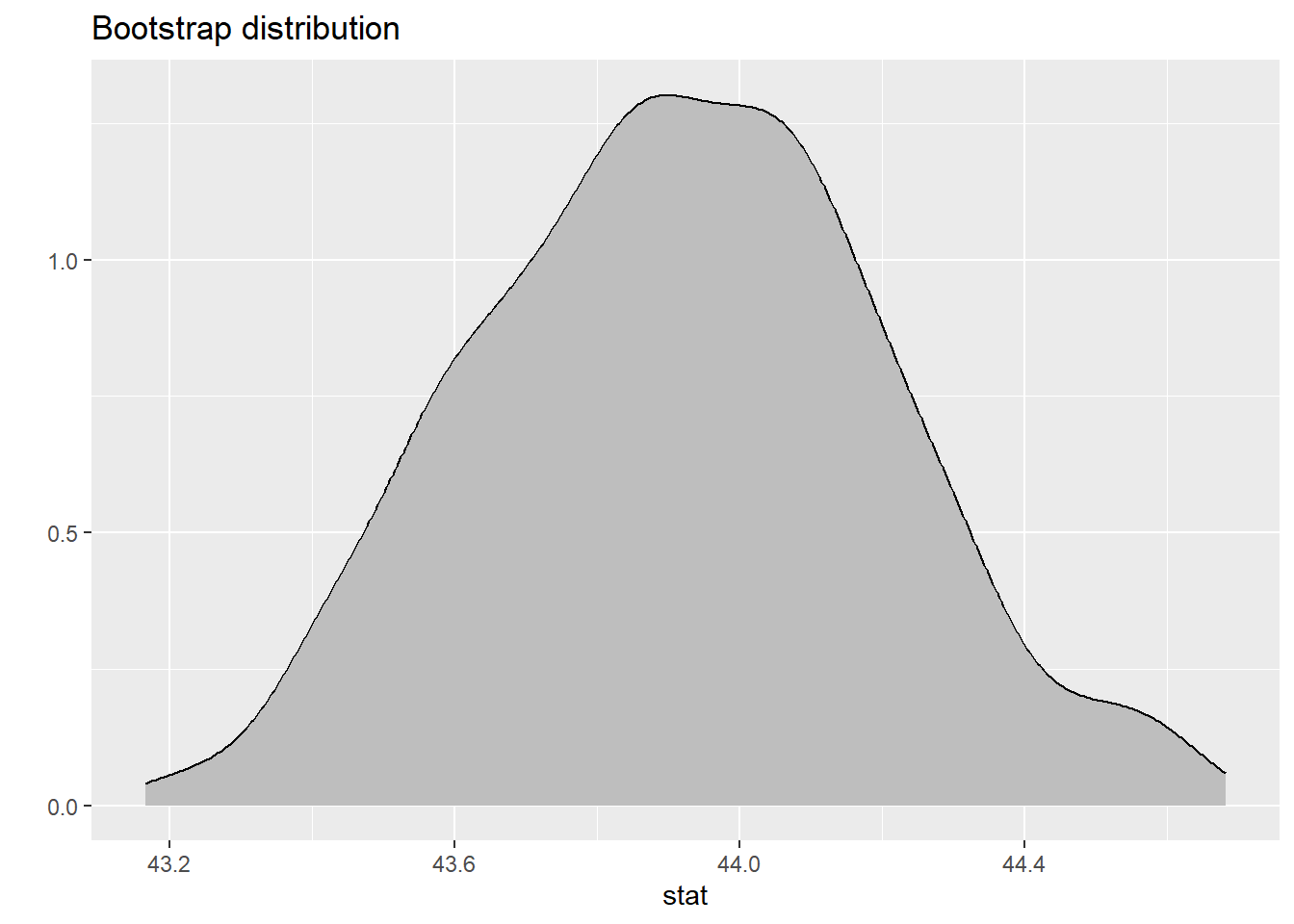
Because we can assume that the assumptions are valid for the central limit theorem, we are going to use simulation based techniques to estimate the true mean bill length of penguins.

See the slides for the steps on how the simulated sampling distribution is created. Below is the code to create this distribution.

The Process

set.seed(12345)

boot_df <- penguins |>
  specify(response = bill_length_mm) |>
  generate(reps = 1000, type = "bootstrap") |>
  calculate(stat = "mean")

Warning: Removed 2 rows containing missing values.

The Graph

boot_df |>
  ggplot(
    aes(x = stat)
  ) + 
  geom_density(fill = "gray") +
  labs(title = "Bootstrap distribution",
       y = "")

The Calculation

boot_df |>
  summarize(lower = quantile(stat, 0.025),
            upper = quantile(stat, 0.975))

# A tibble: 1 × 2
  lower upper
  <dbl> <dbl>
1  43.4  44.5