Random Variables & Probability Distributions
Packages
First, we are going to create a probability distribution by hand. Suppose that our random variable is the following:
\[ X =\text{number of times three coins lands on heads}\\ \]
Is this discrete or continuous?
add text
Now, in order to calculate our probability distribution, let’s think about all possibilities of our three coins. Write them out below.
data <- tribble(
  ~heads, ~percentage,
  "0",   1/8,
  "1",   3/8,
  "2",   3/8,
  "3",   1/8
)

data
# A tibble: 4 × 2
heads percentage
<chr> <dbl>
1 0 0.125
2 1 0.375
3 2 0.375
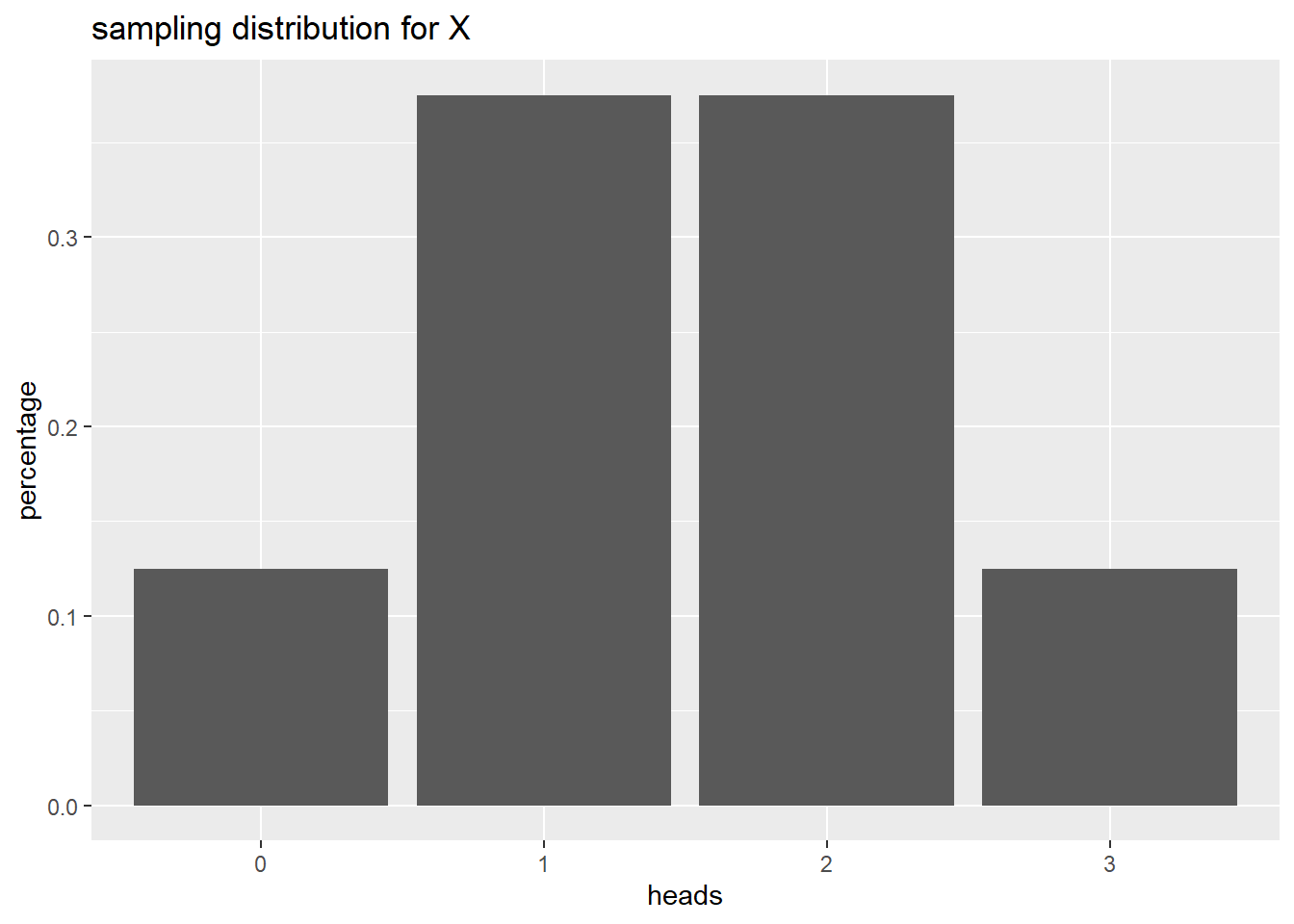
4 3 0.125Now, let’s use the appropriate geom to plot the probability distribution.
data |>
  ggplot(aes(x = heads, y = percentage)) +
  geom_col() +
  labs(title = "sampling distribution for X")
Calculating probabilities
We can use this information to calculate probabilities!
– What’s the probability that 0 coins land on heads? What is the proper notation for this probability?
P(X = 0) = 0.125
– What’s the probability that at least one coin lands on heads? What is the proper notation for this probability?
P(X > 0) = 0.375 + 0.375 + 0.125
– What’s the probability that two or more coins land on heads? What is the proper notation for this probability?
P(X > 1) = 0.375 + 0.125
Continuous Probability Distribution
What is a continuous random variable?
A continuous random variable is one which takes an infinite number of possible values.
The data
times <- read_csv("https://st511-01.github.io/data/times.csv")Rows: 10000 Columns: 1
── Column specification ────────────────────────────────────────────────────────
Delimiter: ","
dbl (1): time_sec
ℹ Use `spec()` to retrieve the full column specification for this data.
ℹ Specify the column types or set `show_col_types = FALSE` to quiet this message.For this next exercise, we are going to look at:
\[ Y =\text{time to complete an IQ test}\\ \]
The Normal Distribution
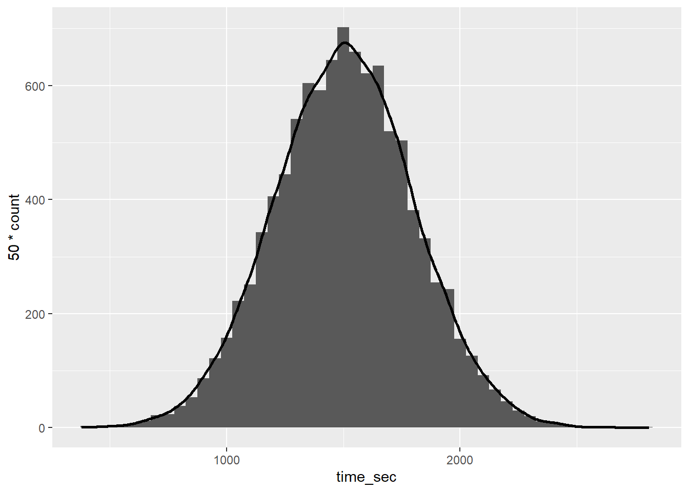
There are many different types of distributions. For this class, we are going to focus on the most common one, the Normal distribution. Suppose that the times are normally distributed, and we have access to the entire population of data (which is not always realistic). Let’s plot the population distribution of times. Further, let’s calculate the population mean and standard deviation of times below.
times |>
  ggplot(
    aes(x = time_sec)
  ) +
  geom_histogram(binwidth = 50, alpha = 1)+
  geom_density(aes(y=50 * ..count..), linewidth = 1 )
Warning: The dot-dot notation (`..count..`) was deprecated in ggplot2 3.4.0.
ℹ Please use `after_stat(count)` instead.
# A tibble: 1 × 2
  center    sd
   <dbl> <dbl>
1  1504.  298.
What is the center of the distribution? What’s the standard deviation of this distribution? Is it skewed?
Center = 1504
Spread = 298
The notation for times being normally distributed is:
X ~ N(1504, 298)
When calculating probabilities, we need to note that:
Probability can be thought of as area under the curve
Probability at any one point is equal to 0
- What is the probability that a random person takes more than 2100 seconds?
- What is the probability that a random student takes less than 1200 seconds?
Sampling Distributions
A probability distribution describes the likelihood of all possible values a random variable can take within a population, while a sampling distribution is the probability distribution of a sample statistic (like the mean), calculated from repeated random samples taken from that population.
In order the calculate a sample statistic, we need to take a sample! Let’s take a random sample of 100 times from the population data and check the mean.
[1] 1569.56How does the mean of the sample compare to the population distribution?
It’s close to 1504, but different.
[1] 1569.56What about the second sample?
Same thing. Close, but different. It’s very important to note that this is also NOT the same as the first sample mean we took! This is the idea of sampling variability.
Let’s take many many samples to create a sampling distribution!
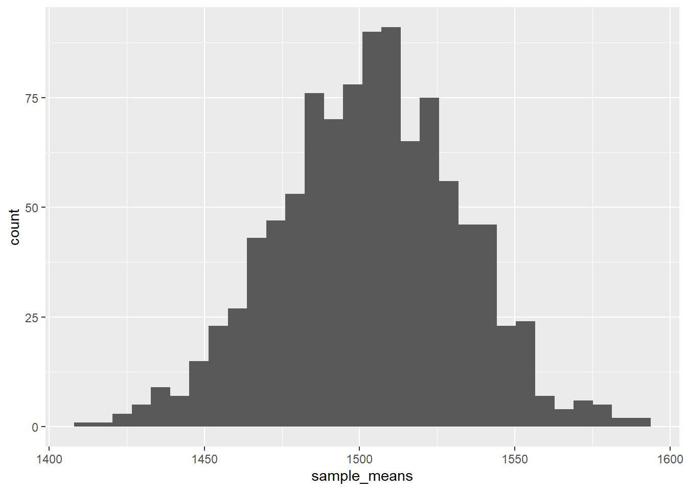
How does the sampling distribution compare to the probability distribution? Plot the sample means + calculate the mean and standard error
sample_means |>
  ggplot(
    aes(x = sample_means)
  ) +
  geom_histogram()
`stat_bin()` using `bins = 30`. Pick better value with `binwidth`.
# A tibble: 1 × 2
  center    sd
   <dbl> <dbl>
1  1503.  29.3
The mean is the same as the population mean (rounding error / need more simulations). The standard error is smaller than the standard deviation of the population distribution by \(\sqrt{n}\)
Using the sampling distribution.
Why do we care?
Sampling distributions help us quantify variability around our statistic
Set the groundwork for statistical inference (hypothesis testing + confidence intervals)
