HW 6 - Interaction Models: Solutions
Packages
Data
For the first, we will be using the lego_sample dataset, which includes data about Lego sets on sale on Amazon.
lego_sample <- read_csv("data/lego_sample.csv")We are going to use the following three variables:
amazon_price: the price for the Lego set listed on Amazon;pieces: the number of Lego pieces in the set;theme: the category the set belongs to.
Exercise-1: Interaction model output
a. Fit an interaction model with theme and number of pieces as your explanatory variables to investigate Amazon price. Name this model price_fit_int. Report your model output below.
Call:
lm(formula = amazon_price ~ pieces * theme, data = lego_sample)

Residuals:
    Min      1Q  Median      3Q     Max
-41.683  -9.851  -3.566   4.961  90.741

Coefficients:
                     Estimate Std. Error t value Pr(>|t|)
(Intercept)          9.437468   6.528891   1.445    0.153
pieces               0.130469   0.018315   7.124 7.94e-10 ***
themeDUPLO®          0.117102   9.117357   0.013    0.990
themeFriends        -6.034602   9.546438  -0.632    0.529
pieces:themeDUPLO®   0.583630   0.140334   4.159 9.05e-05 ***
pieces:themeFriends -0.004644   0.027071  -0.172    0.864
---
Signif. codes:  0 '***' 0.001 '**' 0.01 '*' 0.05 '.' 0.1 ' ' 1

Residual standard error: 20.81 on 69 degrees of freedom
Multiple R-squared:  0.6358,    Adjusted R-squared:  0.6094
F-statistic: 24.09 on 5 and 69 DF,  p-value: 6.12e-14
b. Write out the entire estimated model in proper notation.
\(\hat{price} = 9.43 + .13*pieces + .117*DUPLO - 6.03*Friends + .584*pieces*DUPLO - 0.005*pieces*Friends\)
c. Write out the estimated model for the DUPLO theme in proper notation.
\(\hat{price} = 9.547 + .714*pieces\)
d. Write out the estimated model for the City theme in proper notation.
\(\hat{price} = 9.43 + .13*pieces\)
e. Without any calculations, justify if the coefficient of determination for the price_fit_int model will be larger, smaller, or not enough information to know, than the coefficient of determination for an additive model with theme and pieces as explanatory variables, and amazon price as the response.
The \(R^2\) will be higher for the interaction model vs the additive model, because the interaction model has the same variables as the additive model, but has more coefficients (is more complicated).
f. Without any calculations, justify if the coefficient of determination for the price_fit_int model will be larger, smaller, or not enough information to know, than the coefficient of determination for an additive model with theme and pieces as explanatory variables, and pages of the manual as the response.
We don’t know if \(R^2\) will be higher or lower. The response variable is different.
Exercise-2: Should we fit a lm?
Data
Gapminder is a “fact tank” that uses publicly available world data to produce data visualizations and teaching resources on global development. We will use an excerpt of their data to explore relationships among world health metrics across countries and regions between the years 1952 and 2007. The data set is called gapminder, from the gapminder package. A table of variables can be found below.
We are going to use the data just from the year 2007 using the following code.
gapminder_2007 <- gapminder |>
  filter(year == 2007) |>
  droplevels()
Use the gapminder_2007 data set to answer the follow questions.
Hint: pull up the help file for gapminder for a variable name key.
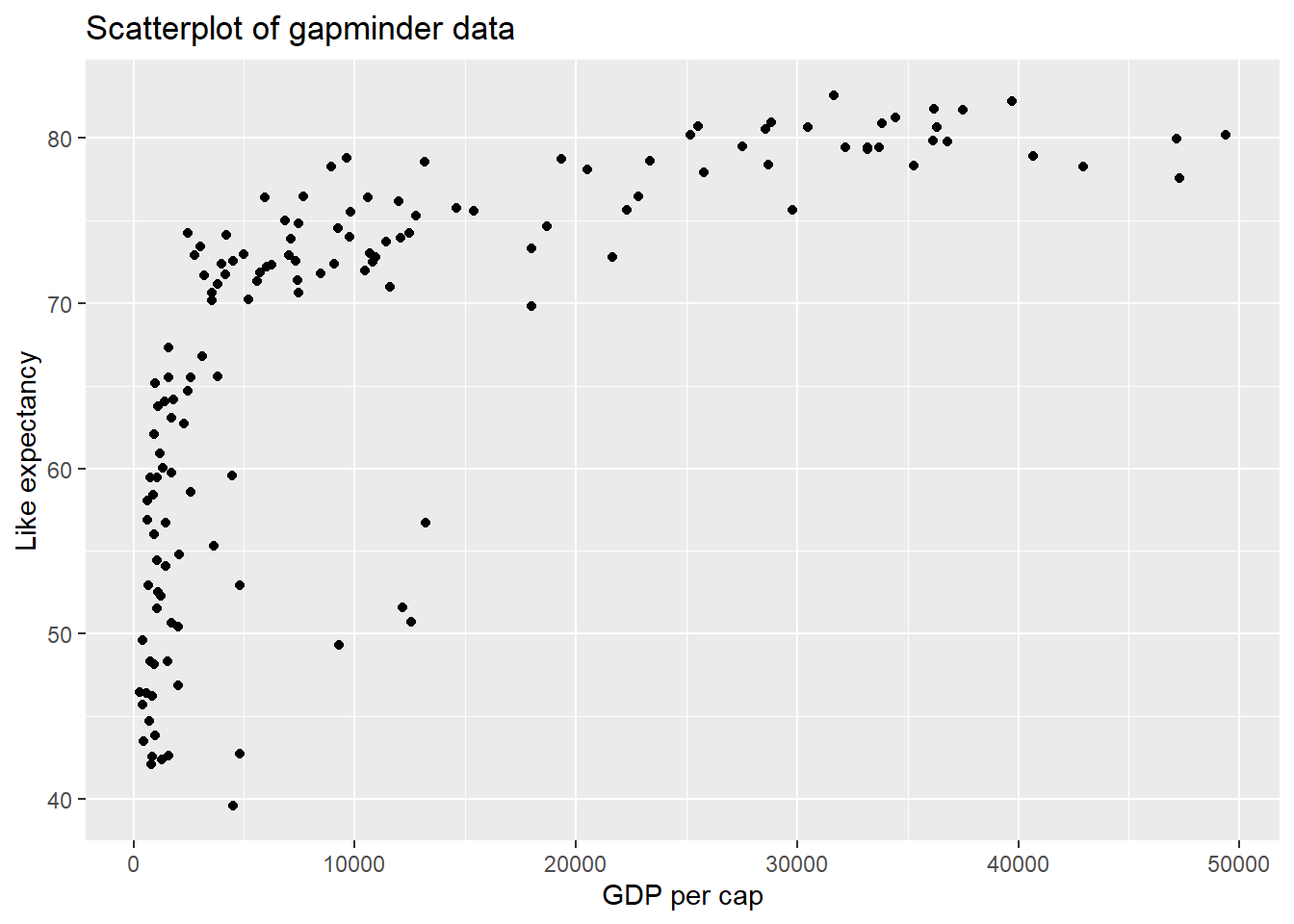
- We are interested in learning more about life expectancy (y), and we’ll start with exploring the relationship between life expectancy and GDP (x). Create a scatter plot of
gdpPercapvs.lifeExp.
gapminder_2007 |>
  ggplot(
    aes(x = gdpPercap, y = lifeExp)
  ) +
  geom_point() +
  labs(x = "GDP per cap",
       y = "Like expectancy",
       title = "Scatterplot of gapminder data")
- While working with a fellow student, they claim that they don’t think it’s appropriate to fit a linear model to explore this relationship. In 1-2 sentences, explain why your fellow student is correct.
There is not a linear relationship between life expectancy and GDP. Therfore, the student is correct, and this relationship should not be studied using a linear model.
- Because of the concern your fellow student raised, we are going to take the natural log of
gdpPercap, and use this as our new response variable (lnDGP) using the following code below.
For the remainder of this question, we are going to use the gapminder_2007_log data set.
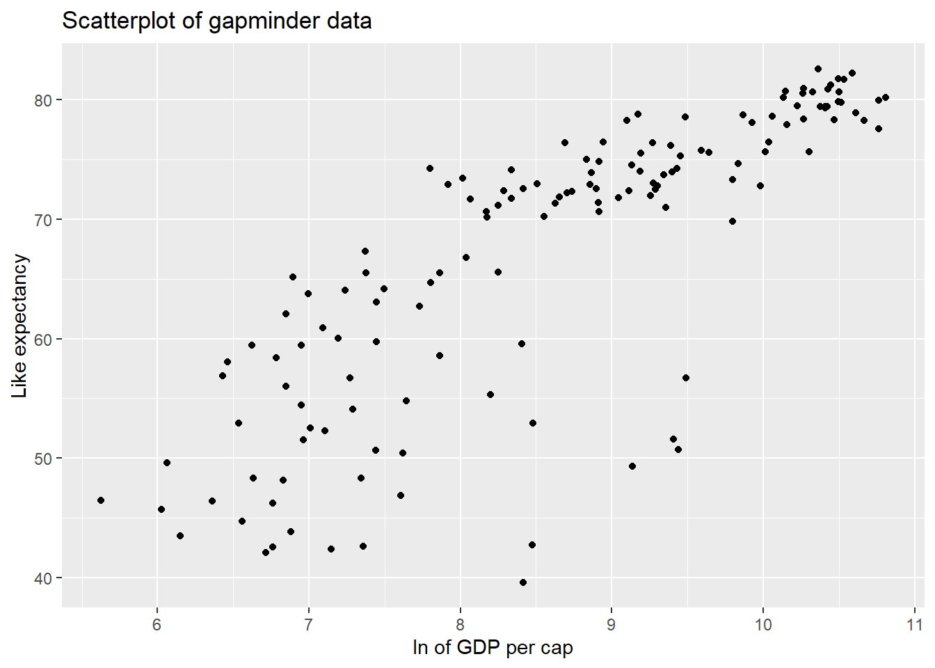
Create a scatter plot of lnGDP vs. lifeExp. Then, make a comment on if you think it is appropriate to fit a linear model to analyze this relationship.
gapminder_2007_log |>
  ggplot(
    aes(x = lnGDP, y = lifeExp)
  ) +
  geom_point() +
  labs(x = "ln of GDP per cap",
       y = "Like expectancy",
       title = "Scatterplot of gapminder data")
It is more appropriate to model the the ln of GDP per cap by life expectancy with a linear model, as there appears to be some evidence of a linear relationship between the two variables (although still a slight curve).
Exercise-3: Model selection
Another student comes to you and suggests that they believe continent could also be a useful variable at explaining the variability in lnGDP. In this exercise, we are going to investigate which model would be the most appropriate to model lnGDP.
-
Using the
gapminder_2007_logdata set, fit the three models below, and report their summary output.SLR model with
lifeExpas the explanatory varaibleAdditive model with
lifeExpandcontinentInteraction model with
lifeExpandcontinent
Call:
lm(formula = lifeExp ~ lnGDP, data = gapminder_2007_log)

Residuals:
    Min      1Q  Median      3Q     Max
-25.947  -2.661   1.215   4.469  13.115

Coefficients:
            Estimate Std. Error t value Pr(>|t|)
(Intercept)   4.9496     3.8577   1.283    0.202
lnGDP         7.2028     0.4423  16.283   <2e-16 ***
---
Signif. codes:  0 '***' 0.001 '**' 0.01 '*' 0.05 '.' 0.1 ' ' 1

Residual standard error: 7.122 on 140 degrees of freedom
Multiple R-squared:  0.6544,    Adjusted R-squared:  0.652
F-statistic: 265.2 on 1 and 140 DF,  p-value: < 2.2e-16
Call:
lm(formula = lifeExp ~ lnGDP + continent, data = gapminder_2007_log)

Residuals:
     Min       1Q   Median       3Q      Max
-19.4917  -2.3146  -0.0432   2.5498  14.8818

Coefficients:
                  Estimate Std. Error t value Pr(>|t|)
(Intercept)        20.1376     4.0332   4.993 1.79e-06 ***
lnGDP               4.6308     0.5274   8.780 6.14e-15 ***
continentAmericas  11.6942     1.6546   7.068 7.46e-11 ***
continentAsia      10.1144     1.4761   6.852 2.31e-10 ***
continentEurope    11.2682     1.8936   5.951 2.14e-08 ***
continentOceania   12.9293     4.5211   2.860  0.00491 **
---
Signif. codes:  0 '***' 0.001 '**' 0.01 '*' 0.05 '.' 0.1 ' ' 1

Residual standard error: 5.929 on 136 degrees of freedom
Multiple R-squared:  0.7674,    Adjusted R-squared:  0.7588
F-statistic: 89.72 on 5 and 136 DF,  p-value: < 2.2e-16
Call:
lm(formula = lifeExp ~ lnGDP * continent, data = gapminder_2007_log)

Residuals:
     Min       1Q   Median       3Q      Max
-19.1483  -2.4726  -0.0517   2.2124  15.4213

Coefficients:
                         Estimate Std. Error t value Pr(>|t|)
(Intercept)              22.90682    6.22285   3.681 0.000337 ***
lnGDP                     4.26088    0.82373   5.173 8.36e-07 ***
continentAmericas        10.15826   15.68051   0.648 0.518222
continentAsia             2.74329    9.80627   0.280 0.780108
continentEurope          12.53213   19.92268   0.629 0.530411
continentOceania         23.89890  279.39987   0.086 0.931964
lnGDP:continentAmericas   0.23319    1.79057   0.130 0.896581
lnGDP:continentAsia       0.89638    1.18998   0.753 0.452625
lnGDP:continentEurope    -0.03398    2.06360  -0.016 0.986886
lnGDP:continentOceania   -0.96521   27.15408  -0.036 0.971698
---
Signif. codes:  0 '***' 0.001 '**' 0.01 '*' 0.05 '.' 0.1 ' ' 1

Residual standard error: 6.004 on 132 degrees of freedom
Multiple R-squared:  0.7685,    Adjusted R-squared:  0.7527
F-statistic: 48.68 on 9 and 132 DF, p-value: < 2.2e-16- Now, using adjusted r-squared, determine what model (of the three models fit) is the “best” model to model life expectancy.
summary(slr)$adj.r.squared[1] 0.6519808summary(add)$adj.r.squared[1] 0.7588141summary(int)$adj.r.squared[1] 0.7526912Based on the adjusted-r-squared value, it appears that the additive model with ln GDP and continent is the most appropriate.
c). Based on your answer to part b, select the most appropriate interpretation of your model below…
Our model suggests that the relationship between ln of GDP per cap and life expectancy does not depend on continent.
Our model suggests that the relationship between ln of GDP per cap and life expectancy does depend on continent.
1
Exercise-4
I hope you enjoyed this question :). Communicating results is extremely important, and we can use power tools to engage an audience when telling a story.
Communication is a critical yet often overlooked part of research. When we engage with our audience and capture their interest, we can ultimately better communicate what we are trying to share.
Please watch the following video: Hans Rosling: 200 years in 4 minutes.
Then, write a paragraph (4-5 sentences) addressing the following:
What did you enjoy about the presentation of data? What did you find interesting
Were there any aspects of the presentation that were hard to follow? If so, what?
What are your general takeaways from this presentation?
What are your general takeaways from how this presentation was given?
